Generators

This tutorial covers generator modeling in PyPSA-GB, including thermal plants, renewable generators, and the dispatch optimization process.

What You’ll Learn

• Generator types and data sources

• Thermal generator characteristics

• Renewable generator profiles

• Dispatch optimization and merit order

• Capacity factors and utilization

1. Setup

import pypsa
import pandas as pd
import numpy as np
import matplotlib.pyplot as plt
import warnings
import folium
from pyproj import Transformer
from _map_utils import prepare_map_network, explore_network_map

warnings.filterwarnings('ignore')
plt.style.use('seaborn-v0_8-whitegrid')
plt.rcParams['figure.figsize'] = [12, 6]
plt.rcParams['figure.dpi'] = 100

# Color definitions
colors = {
    'CCGT': '#FF6B35', 'CCGT_hydrogen': '#FF9966', 'nuclear': '#E91E63',
    'coal': '#424242', 'wind_onshore': '#3B6182', 'wind_offshore': '#6BAED6',
    'solar_pv': '#FFBB00', 'biomass': '#4CAF50', 'large_hydro': '#0868AC',
    'small_hydro': '#08519C', 'OCGT': '#FF9800', 'marine': '#00BCD4',
    'oil': '#795548', 'load_shedding': '#F44336'
}

print(f"PyPSA version: {pypsa.__version__}")

PyPSA version: 1.0.7

2. Generator Data Sources

Source	Type	Used For
DUKES	Official UK stats	Historical thermal capacity
REPD	Planning database	Renewable sites and capacity
FES	Future scenarios	Future capacity projections
TEC Register	Grid connections	Large generator verification

3. Load a Network

# Load network
n = pypsa.Network("../../../resources/network/HT35_clustered_solved.nc")

print(f"Network loaded")
print(f"  Total generators: {len(n.generators)}")
print(f"  Unique carriers: {n.generators.carrier.nunique()}")
print(f"  Snapshots: {len(n.snapshots)}")

INFO:pypsa.network.io:Imported network 'HT35_clustered (Clustered)' has buses, carriers, generators, lines, links, loads, storage_units, stores, sub_networks

Network loaded
  Total generators: 4941
  Unique carriers: 20
  Snapshots: 168

4. Generator Structure

4.1 Generator Attributes

# Generator DataFrame
print("Generator columns:")
print(n.generators.columns.tolist())

print(f"\nKey attributes:")
print("  - bus: Connection point")
print("  - carrier: Technology type")
print("  - p_nom: Nominal capacity (MW)")
print("  - marginal_cost: Cost per MWh")
print("  - efficiency: Conversion efficiency")

Generator columns:
['bus', 'control', 'type', 'p_nom', 'p_nom_mod', 'p_nom_extendable', 'p_nom_min', 'p_nom_max', 'p_nom_set', 'p_min_pu', 'p_max_pu', 'p_set', 'e_sum_min', 'e_sum_max', 'q_set', 'sign', 'carrier', 'marginal_cost', 'marginal_cost_quadratic', 'active', 'build_year', 'lifetime', 'capital_cost', 'efficiency', 'committable', 'start_up_cost', 'shut_down_cost', 'stand_by_cost', 'min_up_time', 'min_down_time', 'up_time_before', 'down_time_before', 'ramp_limit_up', 'ramp_limit_down', 'ramp_limit_start_up', 'ramp_limit_shut_down', 'weight', 'p_nom_opt', 'lon', 'lat', 'data_source', 'country', 'source']

Key attributes:
  - bus: Connection point
  - carrier: Technology type
  - p_nom: Nominal capacity (MW)
  - marginal_cost: Cost per MWh
  - efficiency: Conversion efficiency

# Sample generators
n.generators[['bus', 'carrier', 'p_nom', 'marginal_cost', 'efficiency']].head(10)

	bus	carrier	p_nom	marginal_cost	efficiency
name
FES_large_hydro_Abham_2035	ABHA1	large_hydro	1.917000	7.04	1.0
FES_large_hydro_Abernethy_2035	ABNE_P	large_hydro	1.475000	7.04	1.0
FES_large_hydro_Alness_2035	ALNE_P	large_hydro	6.153000	7.04	1.0
FES_large_hydro_Alverdiscott_2035	ALVE1	large_hydro	2.486000	7.04	1.0
FES_large_hydro_Ardkinglas_2035	ARDK_P|CLAC_P	large_hydro	4.661000	7.04	1.0
FES_large_hydro_Ardmore_2035	DUGR_P	large_hydro	0.139000	7.04	1.0
FES_large_hydro_Axminster_2035	AXMI1	large_hydro	0.048000	7.04	1.0
FES_large_hydro_Beauly_2035	BEAU_P|ORRI_P	large_hydro	20.872000	7.04	1.0
FES_large_hydro_DirectSHETL_BEAU1J_2035	BEAU_P|ORRI_P	large_hydro	109.857879	7.04	1.0
FES_large_hydro_Beddington_SPN_2035	BEDD_1	large_hydro	0.837000	7.04	1.0

4.2 Capacity by Technology

# Installed capacity by carrier
capacity = n.generators.groupby('carrier')['p_nom'].sum().sort_values(ascending=False)
capacity_gw = capacity / 1000

print("Installed Capacity (GW):")
print(capacity_gw.round(2).to_string())
print(f"\nTotal: {capacity_gw.sum():.2f} GW")

Installed Capacity (GW):
carrier
wind_offshore       88.55
load_shedding       82.05
solar_pv            69.19
wind_onshore        31.12
EU_import           26.02
CCGT                 6.84
nuclear              5.00
advanced_biofuel     4.96
biomass              4.96
waste_to_energy      4.24
large_hydro          1.91
biogas               1.70
OCGT                 0.88
landfill_gas         0.86
CHP                  0.48
gas_engine           0.46
marine               0.34
oil                  0.08
sewage_gas           0.06
geothermal           0.01

Total: 329.70 GW

# Capacity bar chart
fig, ax = plt.subplots(figsize=(12, 6))

carrier_colors = [colors.get(c, '#888888') for c in capacity_gw.index]
capacity_gw.plot(kind='bar', ax=ax, color=carrier_colors, edgecolor='black')

ax.set_ylabel('Capacity (GW)')
ax.set_xlabel('Technology')
ax.set_title('Installed Generation Capacity')
ax.tick_params(axis='x', rotation=45)

plt.tight_layout()
plt.show()

5. Thermal Generators

5.1 Characteristics

# Thermal generator types
thermal_carriers = ['CCGT', 'coal', 'OCGT', 'nuclear', 'biomass', 'oil']
thermal_gens = n.generators[n.generators.carrier.isin(thermal_carriers)]

print(f"Thermal Generators: {len(thermal_gens)}")
print(f"\nCapacity by type (GW):")
print(thermal_gens.groupby('carrier')['p_nom'].sum().sort_values(ascending=False) / 1000)

Thermal Generators: 178

Capacity by type (GW):
carrier
CCGT       6.840000
nuclear    5.000000
biomass    4.961803
OCGT       0.878900
oil        0.078500
Name: p_nom, dtype: float64

# Efficiency and marginal costs
thermal_stats = thermal_gens.groupby('carrier').agg({
    'p_nom': 'sum',
    'efficiency': 'mean',
    'marginal_cost': 'mean'
}).round(2)
thermal_stats.columns = ['Capacity (MW)', 'Avg Efficiency', 'Avg Marginal Cost (£/MWh)']

print("Thermal Generator Characteristics:")
thermal_stats

Thermal Generator Characteristics:

	Capacity (MW)	Avg Efficiency	Avg Marginal Cost (£/MWh)
carrier
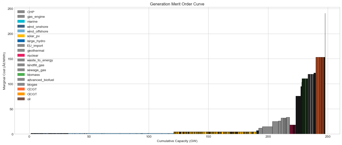
CCGT	6840.0	0.5	152.96
OCGT	878.9	0.5	152.96
biomass	4961.8	0.5	110.40
nuclear	5000.0	0.5	18.04
oil	78.5	0.5	240.61

5.2 Merit Order

# Merit order curve
gen_costs = n.generators[['carrier', 'p_nom', 'marginal_cost']].copy()
gen_costs = gen_costs[gen_costs.marginal_cost < 1000]  # Exclude load shedding
gen_costs = gen_costs.sort_values('marginal_cost')
gen_costs['cumulative_capacity'] = gen_costs['p_nom'].cumsum() / 1000  # GW

fig, ax = plt.subplots(figsize=(14, 6))

prev_cap = 0
for carrier in gen_costs.carrier.unique():
    carrier_gens = gen_costs[gen_costs.carrier == carrier]
    for _, gen in carrier_gens.iterrows():
        ax.bar(prev_cap + gen['p_nom']/2000, gen['marginal_cost'],
               width=gen['p_nom']/1000, color=colors.get(carrier, '#888888'),
               edgecolor='black', linewidth=0.5)
        prev_cap += gen['p_nom']/1000

# Legend
handles = [plt.Rectangle((0,0),1,1, color=colors.get(c, '#888888'))
           for c in gen_costs.carrier.unique()]
ax.legend(handles, gen_costs.carrier.unique(), loc='upper left')

ax.set_xlabel('Cumulative Capacity (GW)')
ax.set_ylabel('Marginal Cost (£/MWh)')
ax.set_title('Generation Merit Order Curve')

plt.tight_layout()
plt.show()

6. Renewable Generators

6.1 Capacity Profiles

# Renewable generators
renewable_carriers = ['wind_onshore', 'wind_offshore', 'solar_pv', 'large_hydro', 'small_hydro']
renewable_gens = n.generators[n.generators.carrier.isin(renewable_carriers)]

print(f"Renewable Generators: {len(renewable_gens)}")
print(f"\nCapacity by type (GW):")
print(renewable_gens.groupby('carrier')['p_nom'].sum().sort_values(ascending=False) / 1000)

Renewable Generators: 1340

Capacity by type (GW):
carrier
wind_offshore    88.553202
solar_pv         69.185866
wind_onshore     31.121222
large_hydro       1.914408
Name: p_nom, dtype: float64

# Check for availability time series
if 'p_max_pu' in n.generators_t:
    print("Availability profiles (p_max_pu) available")

    # Sample availability for each carrier
    for carrier in renewable_carriers:
        carrier_gens = n.generators[n.generators.carrier == carrier].index
        if len(carrier_gens) > 0:
            # Get first generator of this type that has a profile
            for gen in carrier_gens:
                if gen in n.generators_t.p_max_pu.columns:
                    cf = n.generators_t.p_max_pu[gen].mean()
                    print(f"  {carrier}: avg CF = {cf*100:.1f}%")
                    break
else:
    print("No availability profiles found")

Availability profiles (p_max_pu) available
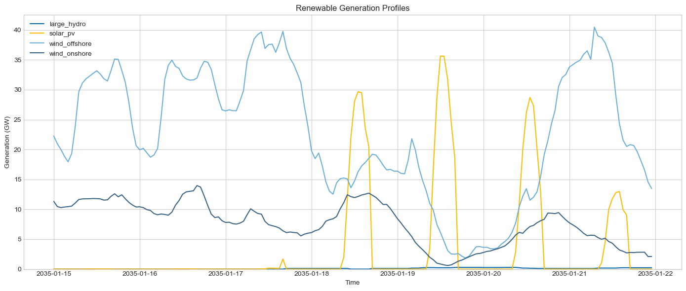
  wind_onshore: avg CF = 42.8%
  wind_offshore: avg CF = 51.6%
  solar_pv: avg CF = 9.6%
  large_hydro: avg CF = 40.0%

6.2 Renewable Output Profiles

# Generation profiles by renewable type
renewable_gen = n.generators_t.p[[g for g in renewable_gens.index if g in n.generators_t.p.columns]]

if len(renewable_gen.columns) > 0:
    # Aggregate by carrier
    gen_by_carrier = renewable_gen.groupby(n.generators.loc[renewable_gen.columns, 'carrier'], axis=1).sum() / 1000

    fig, ax = plt.subplots(figsize=(14, 6))

    for carrier in gen_by_carrier.columns:
        ax.plot(gen_by_carrier.index, gen_by_carrier[carrier],
               label=carrier, linewidth=1.5, color=colors.get(carrier, '#888888'))

    ax.set_ylabel('Generation (GW)')
    ax.set_xlabel('Time')
    ax.set_title('Renewable Generation Profiles')
    ax.legend()
    ax.set_ylim(bottom=0)

    plt.tight_layout()
    plt.show()

7. Generator Spatial Distribution

# Capacity by bus
bus_capacity = n.generators.groupby('bus')['p_nom'].sum() / 1000  # GW

map_n = prepare_map_network(n)
map_n.buses["capacity_GW"] = bus_capacity.reindex(map_n.buses.index).fillna(0)

print("Generation Capacity Distribution (Bus size = capacity)")
print("lon range:", float(map_n.buses.x.min()), float(map_n.buses.x.max()))
print("lat range:", float(map_n.buses.y.min()), float(map_n.buses.y.max()))

# Interactive network map with capacity-based bus sizing
m = map_n.plot.explore(
    map_style="light",
    tooltip=True,
    bus_size=map_n.buses["capacity_GW"].clip(lower=0.1) * 1000,
    bus_size_factor=0.05,
    branch_width_factor=1.0,
    bus_columns=["capacity_GW", "v_nom"],
)
m

Generation Capacity Distribution (Bus size = capacity)
lon range: -6.960335346509393 9.1167
lat range: 50.394884755225235 59.349999999999994