Electric Vehicle Flexibility#
This tutorial demonstrates how PyPSA-GB models electric vehicle (EV) demand flexibility, including smart charging, Vehicle-to-Grid (V2G), and different tariff behaviors.
The HT35_flex scenario uses ``flex_share = 0.2``, meaning:
20% of EV demand → Smart charging (optimizable, Store + Link components)
80% of EV demand → Dumb loads (fixed evening-peak profile, merged into base electricity)
This reflects the reality that only a fraction of EV owners have smart chargers or participate in flexibility programs.
Hardware capacities (chargers, batteries, V2G) come directly from FES building blocks (Srg_BB005 for V2G, Srg_BB007a for smart charging).
What You’ll Learn.#
How
flex_sharesplits EV demand between flexible and inflexible. Analyzing charging patterns, V2G dispatch, and battery state of chargeThe four tariff modes (GO, INT, V2G, MIXED) and their PyPSA implementations
1. Setup#
[1]:
import pypsa
import pandas as pd
import numpy as np
import matplotlib.pyplot as plt
import warnings

warnings.filterwarnings('ignore')
plt.style.use('seaborn-v0_8-whitegrid')
plt.rcParams['figure.figsize'] = [14, 6]
plt.rcParams['figure.dpi'] = 100

print(f"PyPSA version: {pypsa.__version__}")
PyPSA version: 1.0.7
[19]:
# Check scenario configuration
import yaml

with open("../../../config/defaults.yaml") as f:
    defaults = yaml.safe_load(f)

with open("../../../config/scenarios.yaml") as f:
    scenarios = yaml.safe_load(f)

ev_defaults = defaults.get('demand_flexibility', {}).get('electric_vehicles', {})
scenario_ev = scenarios.get('HT35_flex', {}).get('demand_flexibility', {}).get('electric_vehicles', {})

print("=" * 70)
print("HT35_FLEX SCENARIO CONFIGURATION")
print("=" * 70)

# Key parameters
eff_flex_share = scenario_ev.get('flex_share', ev_defaults.get('flex_share', 1.0))
eff_tariff = scenario_ev.get('tariff', ev_defaults.get('tariff', 'INT'))
use_fes = ev_defaults.get('v2g', {}).get('use_fes_capacity', True)

print(f"DEMAND SPLIT (flex_share)")
print(f"  flex_share = {eff_flex_share}")
print(f"  ├─ {eff_flex_share*100:.0f}% flexible   → Smart charging (Store + Link components)")
print(f"  └─ {(1-eff_flex_share)*100:.0f}% inflexible → Dumb loads (merged into 'electricity')")

print(f"TARIFF MODE")
print(f"  tariff = '{eff_tariff}'")
if eff_tariff == 'MIXED':
    print(f"  └─ Splits flexible demand across GO/INT/V2G using FES data")
else:
    print(f"  └─ All flexible EVs use {eff_tariff} tariff")

print(f"CAPACITY SOURCE")
print(f"  use_fes_capacity = {use_fes}")
if use_fes:
    print(f"  ├─ V2G:            FES Srg_BB005 (~17.9 GW for HT 2035)")
    print(f"  ├─ Smart charging: FES Srg_BB007a")
    print(f"  └─ Scaled by:      flex_share × tariff mode shares")
else:
    print(f"  └─ Calculated from fleet size × charger power")

print(f"OTHER SETTINGS")
print(f"  battery_capacity_kwh:  {ev_defaults.get('battery_capacity_kwh', 60)} kWh (average EV battery)")
print(f"  charge_efficiency:     {ev_defaults.get('charge_efficiency', 0.9)} (grid-to-battery)")
print(f"  charger_power_kw:      {ev_defaults.get('int', {}).get('charger_power_kw', 7)} kW (home charger)")
print("\n" + "=" * 70)
======================================================================
HT35_FLEX SCENARIO CONFIGURATION
======================================================================
DEMAND SPLIT (flex_share)
  flex_share = 0.2
  ├─ 20% flexible   → Smart charging (Store + Link components)
  └─ 80% inflexible → Dumb loads (merged into 'electricity')
TARIFF MODE
  tariff = 'MIXED'
  └─ Splits flexible demand across GO/INT/V2G using FES data
CAPACITY SOURCE
  use_fes_capacity = True
  ├─ V2G:            FES Srg_BB005 (~17.9 GW for HT 2035)
  ├─ Smart charging: FES Srg_BB007a
  └─ Scaled by:      flex_share × tariff mode shares
OTHER SETTINGS
  battery_capacity_kwh:  60.0 kWh (average EV battery)
  charge_efficiency:     0.9 (grid-to-battery)
  charger_power_kw:      7.0 kW (home charger)

======================================================================
[20]:
# Check all load carriers in the network to find where the 80% dumb EV demand went
n = pypsa.Network("../../../resources/network/HT35_flex_solved.nc")

print("ALL LOAD CARRIERS IN NETWORK:")
print("-" * 60)
for carrier in sorted(n.loads.carrier.unique()):
    loads_c = n.loads[n.loads.carrier == carrier]
    if len(n.loads_t.p_set.columns.intersection(loads_c.index)) > 0:
        total = n.loads_t.p_set[loads_c.index.intersection(n.loads_t.p_set.columns)].sum().sum() / 1000  # GWh
    else:
        total = 0
    print(f"  {carrier:30s}: {len(loads_c):>5} loads, {total:>10.1f} GWh")

# Also check: what fraction of total demand is EV driving?
ev_driving = n.loads[n.loads.carrier == 'EV driving']
ev_demand = n.loads_t.p_set[ev_driving.index].sum().sum() / 1000  # GWh

elec_loads = n.loads[n.loads.carrier == 'electricity']
elec_demand = n.loads_t.p_set[elec_loads.index].sum().sum() / 1000  # GWh

print()
print("DEMAND BREAKDOWN:")
print(f"  Base electricity:  {elec_demand:>10.1f} GWh")
print(f"  EV driving (flex): {ev_demand:>10.1f} GWh")
print(f"  Total:             {elec_demand + ev_demand:>10.1f} GWh")
INFO:pypsa.network.io:Imported network 'HT35_flex (Clustered)' has buses, carriers, generators, lines, links, loads, storage_units, stores, sub_networks
ALL LOAD CARRIERS IN NETWORK:
------------------------------------------------------------
  EV driving                    :   936 loads,      246.7 GWh
  electricity                   :   251 loads,     6013.5 GWh

DEMAND BREAKDOWN:
  Base electricity:      6013.5 GWh
  EV driving (flex):      246.7 GWh
  Total:                 6260.2 GWh
2. Background: Why EV Flexibility Matters#
Electric vehicles represent a major new source of electricity demand in Great Britain. By 2035, FES projects EVs could add 30-60 TWh of electricity demand annually. However, unlike traditional loads, EVs have inherent flexibility:
Battery storage: EVs have large batteries (40-100 kWh) that only need partial daily recharge
Plug-in time >> Charging time: Cars parked 95% of day, charging takes 4-8 hours
Predictable patterns: Regular commuting creates predictable demand and availability
Flexibility value comes from:
Peak shaving: Avoiding expensive evening demand peaks (£100-200/MWh)
Renewable integration: Charging when wind/solar abundant (£30-50/MWh)
Grid services (V2G): Providing balancing during stress (£100-300/MWh)
Transmission relief: Temporal load distribution reduces network congestion
2.1 How PyPSA-GB Models EV Flexibility#
PyPSA-GB uses ``flex_share`` to split EV demand into two groups:
Flexible EVs (20% with
flex_share=0.2): Modeled as Store + Link components that can optimize charging timingInflexible EVs (80%): Modeled as fixed Load components with evening-peak profile
Hardware capacities (chargers, batteries, V2G) come from FES building blocks (Srg_BB005, Srg_BB007a), not calculated from fleet size.
2.2 Four EV Tariff Modes#
PyPSA-GB models four EV flexibility mechanisms, each representing different consumer behaviors:
Mode |
Description |
PyPSA Implementation |
Flexibility Level |
|---|---|---|---|
GO |
Fixed night window (Octopus Go style) |
Store + Link (cost-incentivized) |
Low (time-shifted only) |
INT |
Intelligent smart charging |
Store + Link (charge only) |
Medium (fully optimizable) |
V2G |
Vehicle-to-Grid bidirectional |
Store + 2 Links (charge/discharge) |
High (includes grid export) |
MIXED |
Splits fleet across GO/INT/V2G |
All of the above |
Realistic heterogeneity |
Note: These tariffs only apply to the flexible portion (20% with flex_share=0.2). The remaining 80% are dumb loads regardless of tariff mode.
GO Mode (Octopus Go Style)#
Grid ──▶ [Charging Window 00:00-04:00] ──▶ EV Battery ──▶ Driving
          (Cost-incentivized)
Simple time-of-use tariff with cheap overnight rates
Charging incentivized during window (£0/MWh) vs outside (£100/MWh)
Low flexibility: shifts load to fixed window
INT Mode (Intelligent Tariff)#
                  efficiency
Grid ──▶ [EV Charger Link] ──▶ [EV Battery Store] ──▶ Driving
                90%              (SOC tracking)        (Load)
Smart charging optimizes when to charge within plugged-in hours
Store tracks battery state of charge (SOC)
Minimum SOC constraint (20%) ensures range availability
Target departure SOC (80% at 7am)
V2G Mode (Vehicle-to-Grid)#
                  90%                                    90%
Grid ──▶ [EV Charger] ──▶ [EV Battery Store] ◀── [V2G Discharge] ◀── Grid
          (Link)            (SOC tracking)         (Link)         (export)
                                   │
                                   ▼
                            Driving (Load)
Bidirectional - EVs can charge and discharge to grid
V2G capacity from FES Srg_BB005 (17.9 GW by 2035 in HT scenario)
Battery degradation cost (£50/MWh) discourages excessive cycling
Provides grid balancing during stress periods
MIXED Mode (HT35_flex uses this)#
Splits flexible fleet across GO/INT/V2G based on FES data
GO share: Non-smart chargers (lowest flexibility)
INT share: Smart chargers without V2G
V2G share: Bidirectional chargers (highest flexibility)
Creates separate component sets for each tariff type at each bus
3. Load a Network with EV Flexibility#
[21]:
# Load a solved network with EV flexibility enabled
# HT35_flex: 2035 Holistic Transition with MIXED tariff and flex_share=0.2
# Only 20% of EV demand participates in flexibility (GO/INT/V2G)
# The remaining 80% is embedded in the base 'electricity' loads
n = pypsa.Network("../../../resources/network/HT35_flex_solved.nc")

print("Network loaded")
print(f"  Buses: {len(n.buses)}")
print(f"  Loads: {len(n.loads)}")
print(f"  Links: {len(n.links)}")
print(f"  Stores: {len(n.stores)}")

print(f"  Snapshots: {len(n.snapshots)}")
print(f"  Period: {n.snapshots[0]} to {n.snapshots[-1]}")
INFO:pypsa.network.io:Imported network 'HT35_flex (Clustered)' has buses, carriers, generators, lines, links, loads, storage_units, stores, sub_networks
Network loaded
  Buses: 1234
  Loads: 1187
  Links: 1530
  Stores: 937
  Snapshots: 168
  Period: 2035-01-13 00:00:00 to 2035-01-19 23:00:00
4. EV Components in the Network#
4.1 Identifying EV Components#
[22]:
# EV components are identified by their carrier

# EV Battery Stores (track SOC)
ev_stores = n.stores[n.stores['carrier'] == 'EV battery']
print(f"EV Battery Stores: {len(ev_stores)}")

# EV Charger Links (grid → battery)
ev_chargers = n.links[n.links['carrier'] == 'EV charger']
print(f"EV Charger Links: {len(ev_chargers)}")

# V2G Links (battery → grid) - only present in V2G mode
v2g_links = n.links[n.links['carrier'] == 'V2G']
print(f"V2G Links: {len(v2g_links)}")

# EV Driving Loads (electricity demand for driving)
ev_loads = n.loads[n.loads['carrier'] == 'EV driving']
print(f"EV Driving Loads: {len(ev_loads)}")

# Show sample components
if len(ev_stores) > 0:
    print("\nSample EV Battery Stores:")
    print(ev_stores[['bus', 'carrier', 'e_nom']].head())

if len(v2g_links) > 0:
    print("\nSample V2G Links:")
    print(v2g_links[['bus0', 'bus1', 'carrier', 'p_nom']].head())
EV Battery Stores: 936
EV Charger Links: 936
V2G Links: 312
EV Driving Loads: 936

Sample EV Battery Stores:
                                                          bus     carrier  \
name
CLAC1Q EV fleet battery GO    EV battery_CLAC1Q EV battery GO  EV battery
CLAC1Q EV fleet battery INT  EV battery_CLAC1Q EV battery INT  EV battery
CLAC1Q EV fleet battery V2G  EV battery_CLAC1Q EV battery V2G  EV battery
DUNO1Q EV fleet battery GO    EV battery_DUNO1Q EV battery GO  EV battery
DUNO1Q EV fleet battery INT  EV battery_DUNO1Q EV battery INT  EV battery

                             e_nom
name
CLAC1Q EV fleet battery GO   0.960
CLAC1Q EV fleet battery INT  1.608
CLAC1Q EV fleet battery V2G  0.636
DUNO1Q EV fleet battery GO   0.708
DUNO1Q EV fleet battery INT  1.188

Sample V2G Links:
                                        bus0  \
name
CLAC1Q V2G  EV battery_CLAC1Q EV battery V2G
DUNO1Q V2G  EV battery_DUNO1Q EV battery V2G
DUNO1R V2G  EV battery_DUNO1R EV battery V2G
KEIT3- V2G  EV battery_KEIT3- EV battery V2G
QUOI1- V2G  EV battery_QUOI1- EV battery V2G

                                          bus1 carrier   p_nom
name
CLAC1Q V2G                       ARDK_P|CLAC_P     V2G  0.0742
DUNO1Q V2G                              DUNO_P     V2G  0.0546
DUNO1R V2G                              DUNO_P     V2G  0.0546
KEIT3- V2G  BERB_P|CAIF_P|DALL_P|GLEF_P|KEIT_P     V2G  0.3850
QUOI1- V2G                              QUOI_P     V2G  0.0028
4.2 EV Capacity Summary#
[23]:
# Summarize EV capacity in the network

print("=" * 60)
print("EV FLEET CAPACITY SUMMARY")
print("=" * 60)

if len(ev_stores) > 0:
    total_battery_gwh = ev_stores['e_nom'].sum() / 1000
    print(f"\nEV Battery Storage:")
    print(f"  Total capacity: {total_battery_gwh:.2f} GWh")
    print(f"  Number of buses: {len(ev_stores)}")
    print(f"  Average per bus: {ev_stores['e_nom'].mean():.1f} MWh")

if len(ev_chargers) > 0:
    total_charge_gw = ev_chargers['p_nom'].sum() / 1000
    print(f"\nEV Charging Capacity:")
    print(f"  Total charging power: {total_charge_gw:.2f} GW")
    print(f"  Number of chargers: {len(ev_chargers)}")

if len(v2g_links) > 0:
    total_v2g_gw = v2g_links['p_nom'].sum() / 1000
    print(f"\nV2G Discharge Capacity:")
    print(f"  Total V2G power: {total_v2g_gw:.2f} GW")
    print(f"  Number of V2G-enabled buses: {len(v2g_links)}")
    print(f"  Note: V2G capacity is scaled by flex_share AND the V2G share of MIXED mode")
    print(f"  FES Srg_BB005 full target: ~17.9 GW (before flex_share/mode splitting)")

if len(ev_loads) > 0:
    # Driving demand on EV battery buses (flex_share fraction only)
    total_ev_demand_gwh = n.loads_t.p_set[ev_loads.index].sum().sum() / 1000
    print(f"\nEV Driving Demand (flexible portion):")

    print(f"  Weekly energy: {total_ev_demand_gwh:.1f} GWh")
    print(f"  The remaining {(1-eff_flex_share)*100:.0f}% is embedded in 'electricity' loads")
    print(f"  This is flex_share={eff_flex_share} of total EV demand")
============================================================
EV FLEET CAPACITY SUMMARY
============================================================

EV Battery Storage:
  Total capacity: 21.15 GWh
  Number of buses: 936
  Average per bus: 22.6 MWh

EV Charging Capacity:
  Total charging power: 2.47 GW
  Number of chargers: 936

V2G Discharge Capacity:
  Total V2G power: 0.49 GW
  Number of V2G-enabled buses: 312
  Note: V2G capacity is scaled by flex_share AND the V2G share of MIXED mode
  FES Srg_BB005 full target: ~17.9 GW (before flex_share/mode splitting)

EV Driving Demand (flexible portion):
  Weekly energy: 246.7 GWh
  The remaining 80% is embedded in 'electricity' loads
  This is flex_share=0.2 of total EV demand
5. EV Availability Profile#
EV availability for charging follows GB traffic patterns - EVs are available when parked (inverse of traffic). This creates:
High availability overnight: ~95% plugged in (00:00-06:00)
Morning dip: ~50% plugged in during commute (07:00-09:00)
Daytime recovery: ~75% plugged in (10:00-16:00)
Evening dip: ~60% plugged in during commute (17:00-19:00)
[24]:
# The availability is encoded in the charger Link's p_max_pu time series
# This limits charging to when EVs are plugged in

if len(ev_chargers) > 0 and len(n.links_t.p_max_pu) > 0:
    # Get availability for one charger
    sample_charger = ev_chargers.index[0]

    if sample_charger in n.links_t.p_max_pu.columns:
        avail = n.links_t.p_max_pu[sample_charger]

        # Average by hour of day
        avail_by_hour = avail.groupby(avail.index.hour).mean()

        fig, axes = plt.subplots(1, 2, figsize=(14, 5))

        # Time series (first week)
        week = avail.iloc[:168]  # First week
        axes[0].plot(range(len(week)), week.values, linewidth=1.5, color='blue')
        axes[0].fill_between(range(len(week)), week.values, alpha=0.3, color='blue')
        axes[0].set_ylabel('Availability (fraction plugged in)')
        axes[0].set_xlabel('Hour of week')
        axes[0].set_title('EV Availability - First Week')
        axes[0].set_ylim(0, 1.05)

        # Average daily profile
        axes[1].bar(avail_by_hour.index, avail_by_hour.values, color='green', alpha=0.7)
        axes[1].set_ylabel('Average availability')
        axes[1].set_xlabel('Hour of day')
        axes[1].set_title('Average Daily EV Availability Profile')
        axes[1].set_ylim(0, 1.05)
        axes[1].set_xticks(range(0, 24, 2))

        plt.tight_layout()
        plt.show()

        print(f"\nAvailability Statistics:")
        print(f"  Mean: {avail.mean():.2f}")
        print(f"  Min: {avail.min():.2f} (peak commute)")
        print(f"  Max: {avail.max():.2f} (overnight)")
else:
    print("No availability time series found - check network configuration")
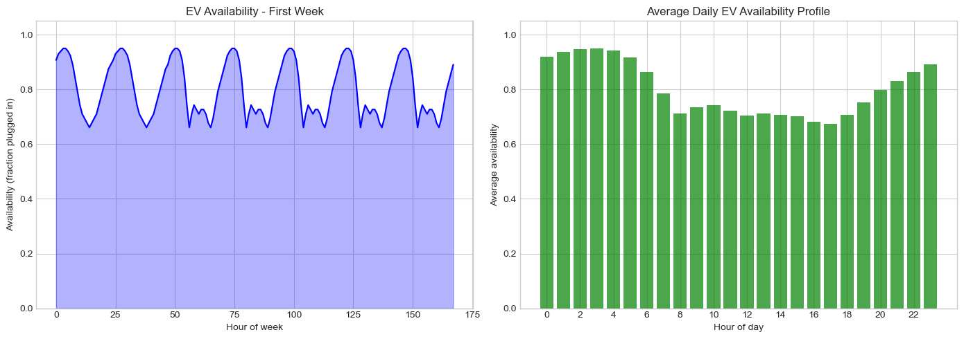
Availability Statistics:
  Mean: 0.80
  Min: 0.66 (peak commute)
  Max: 0.95 (overnight)
6. Analyzing EV Charging Behavior#
6.1 Total EV Charging Profile#
[25]:
# Get total EV charging power from charger links
# p0 is positive when power flows from grid (bus0) to battery (bus1)

if len(ev_chargers) > 0 and len(n.links_t.p0) > 0:
    charger_cols = [c for c in n.links_t.p0.columns if c in ev_chargers.index]

    if charger_cols:
        total_charging = n.links_t.p0[charger_cols].sum(axis=1) / 1000  # GW

        print("EV Charging Statistics:")
        print(f"  Mean charging: {total_charging.mean():.2f} GW")
        print(f"  Peak charging: {total_charging.max():.2f} GW")
        print(f"  Total energy: {total_charging.sum():.0f} GWh")

        # Plot
        fig, ax = plt.subplots(figsize=(14, 5))
        ax.plot(total_charging.index, total_charging.values, linewidth=1.5, color='green')
        ax.fill_between(total_charging.index, total_charging.values, alpha=0.3, color='green')
        ax.axhline(y=total_charging.mean(), color='red', linestyle='--',
                   label=f'Mean: {total_charging.mean():.2f} GW')
        ax.set_ylabel('EV Charging Power (GW)')
        ax.set_xlabel('Time')
        ax.set_title('Total EV Fleet Charging Power')
        ax.legend()
        plt.tight_layout()
        plt.show()
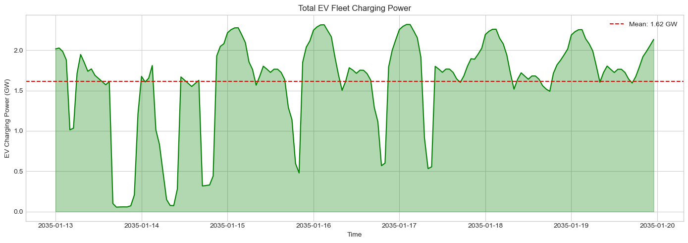
EV Charging Statistics:
  Mean charging: 1.62 GW
  Peak charging: 2.32 GW
  Total energy: 272 GWh
6.2 Daily Charging Pattern#
[26]:
# Average charging by hour of day
if len(ev_chargers) > 0 and len(n.links_t.p0) > 0:
    charger_cols = [c for c in n.links_t.p0.columns if c in ev_chargers.index]

    if charger_cols:
        total_charging = n.links_t.p0[charger_cols].sum(axis=1) / 1000  # GW

        # Group by hour
        charging_by_hour = total_charging.groupby(total_charging.index.hour).mean()

        # Compare with unmanaged (evening peak) profile
        # Typical unmanaged charging peaks 17:00-21:00 when people return home
        unmanaged_profile = np.array([
            0.3, 0.2, 0.2, 0.2, 0.2, 0.3,  # 00:00-05:00 (overnight, low)
            0.4, 0.5, 0.5, 0.5, 0.5, 0.5,  # 06:00-11:00 (morning)
            0.5, 0.5, 0.5, 0.5, 0.6, 0.8,  # 12:00-17:00 (afternoon)
            1.0, 1.0, 0.9, 0.7, 0.5, 0.4   # 18:00-23:00 (evening peak)
        ])
        unmanaged_scaled = unmanaged_profile * charging_by_hour.sum() / unmanaged_profile.sum()

        fig, ax = plt.subplots(figsize=(12, 6))

        width = 0.35
        hours = np.arange(24)

        ax.bar(hours - width/2, charging_by_hour.values, width,
               label='Smart Charging (Optimized)', color='green', alpha=0.7)
        ax.bar(hours + width/2, unmanaged_scaled, width,
               label='Unmanaged (Evening Peak)', color='red', alpha=0.5)

        ax.set_ylabel('Average Charging Power (GW)')
        ax.set_xlabel('Hour of Day')
        ax.set_title('Smart Charging vs Unmanaged Charging Profile')
        ax.set_xticks(hours)
        ax.legend()
        ax.grid(True, alpha=0.3)

        plt.tight_layout()
        plt.show()

        # Calculate peak reduction
        print(f"\nPeak Reduction from Smart Charging:")
        print(f"  Unmanaged evening peak: {unmanaged_scaled.max():.2f} GW")
        print(f"  Smart charging peak: {charging_by_hour.max():.2f} GW")
        print(f"  Peak reduction: {(1 - charging_by_hour.max()/unmanaged_scaled.max())*100:.1f}%")
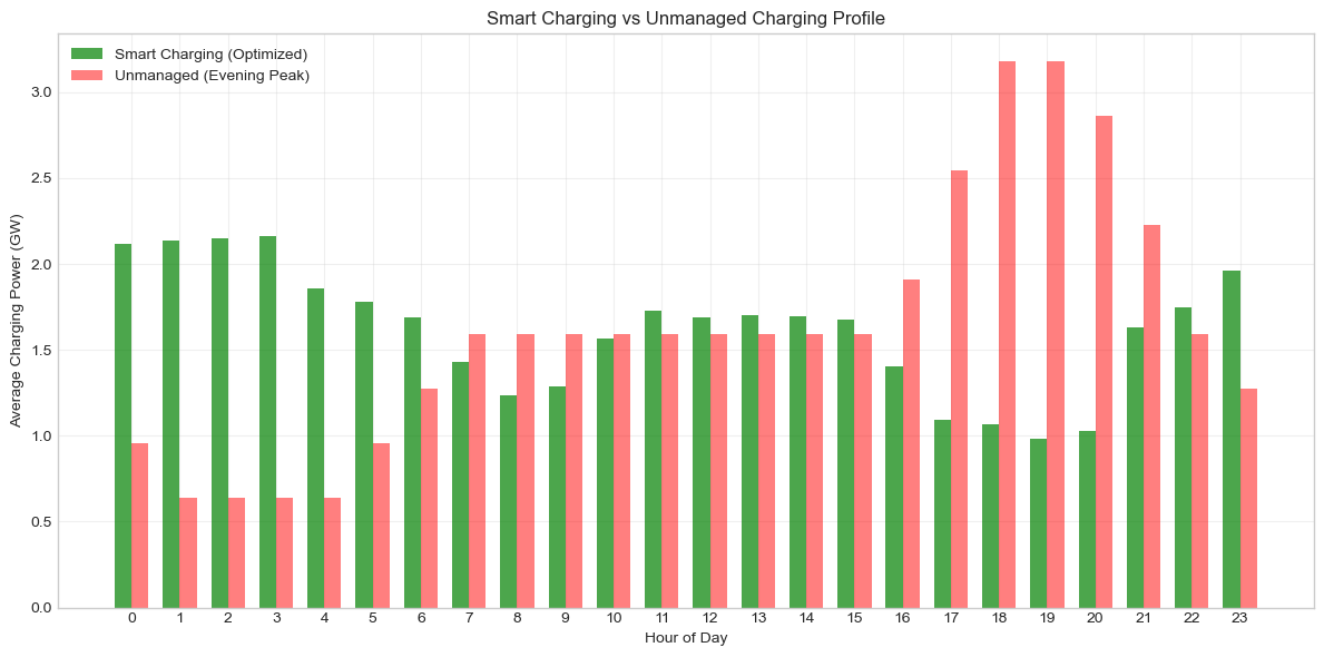
Peak Reduction from Smart Charging:
  Unmanaged evening peak: 3.18 GW
  Smart charging peak: 2.16 GW
  Peak reduction: 32.1%
7. V2G Dispatch Analysis#
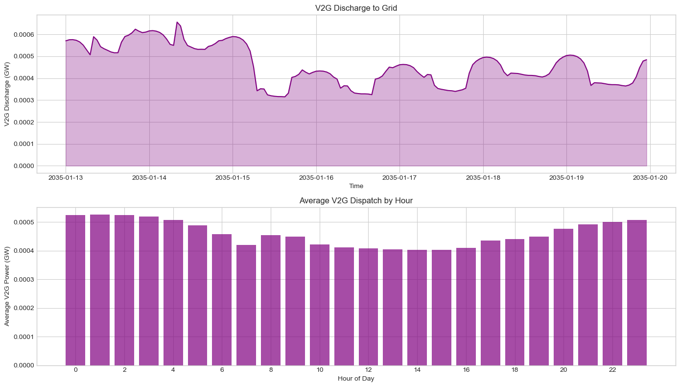
V2G (Vehicle-to-Grid) allows EVs to discharge back to the grid, providing additional flexibility. The optimizer decides when V2G discharge is valuable based on:
System price: Discharge when electricity prices are high
Grid stress: Help during peak demand periods
Battery degradation: Cost of cycling discourages excessive V2G use
[27]:
# Analyze V2G discharge if present
if len(v2g_links) > 0 and len(n.links_t.p0) > 0:
    v2g_cols = [c for c in n.links_t.p0.columns if c in v2g_links.index]

    if v2g_cols:
        # p0 is positive when power flows from battery to grid
        total_v2g = n.links_t.p0[v2g_cols].sum(axis=1) / 1000  # GW

        print("V2G Dispatch Statistics:")
        print(f"  Total V2G energy: {total_v2g.sum():.0f} GWh")
        print(f"  Peak V2G power: {total_v2g.max():.2f} GW")
        print(f"  Hours with V2G > 0: {(total_v2g > 0.001).sum()}")

        # Compare V2G capacity utilization
        total_v2g_capacity = v2g_links['p_nom'].sum() / 1000  # GW
        utilization = total_v2g.max() / total_v2g_capacity * 100 if total_v2g_capacity > 0 else 0
        print(f"  V2G capacity: {total_v2g_capacity:.2f} GW")
        print(f"  Peak utilization: {utilization:.1f}%")

        # Plot V2G dispatch
        fig, axes = plt.subplots(2, 1, figsize=(14, 8), sharex=False)

        # Time series
        axes[0].plot(total_v2g.index, total_v2g.values, linewidth=1.5, color='purple')
        axes[0].fill_between(total_v2g.index, total_v2g.values, alpha=0.3, color='purple')
        axes[0].set_ylabel('V2G Discharge (GW)')
        axes[0].set_xlabel('Time')
        axes[0].set_title('V2G Discharge to Grid')

        # By hour of day
        v2g_by_hour = total_v2g.groupby(total_v2g.index.hour).mean()
        axes[1].bar(v2g_by_hour.index, v2g_by_hour.values, color='purple', alpha=0.7)
        axes[1].set_ylabel('Average V2G Power (GW)')
        axes[1].set_xlabel('Hour of Day')
        axes[1].set_title('Average V2G Dispatch by Hour')
        axes[1].set_xticks(range(0, 24, 2))

        plt.tight_layout()
        plt.show()
else:
    print("No V2G links found - network may be using GO or INT tariff mode")
V2G Dispatch Statistics:
  Total V2G energy: 0 GWh
  Peak V2G power: 0.00 GW
  Hours with V2G > 0: 0
  V2G capacity: 0.49 GW
  Peak utilization: 0.1%
7.1 V2G Value Analysis#
[28]:
# When does V2G discharge? Compare with marginal prices
if len(v2g_links) > 0 and len(n.links_t.p0) > 0 and len(n.buses_t.marginal_price) > 0:
    v2g_cols = [c for c in n.links_t.p0.columns if c in v2g_links.index]

    if v2g_cols:
        total_v2g = n.links_t.p0[v2g_cols].sum(axis=1) / 1000  # GW

        # Get average marginal price across buses
        avg_price = n.buses_t.marginal_price.mean(axis=1)

        # Create comparison DataFrame
        comparison = pd.DataFrame({
            'v2g_gw': total_v2g,
            'price': avg_price
        })

        # Identify V2G active hours
        v2g_active = comparison[comparison['v2g_gw'] > 0.001]

        if len(v2g_active) > 0:
            print("V2G Value Analysis:")
            print(f"  Average price when V2G active: £{v2g_active['price'].mean():.2f}/MWh")
            print(f"  Average price overall: £{avg_price.mean():.2f}/MWh")
            print(f"  Price premium captured: £{v2g_active['price'].mean() - avg_price.mean():.2f}/MWh")

            # Plot price vs V2G
            fig, ax1 = plt.subplots(figsize=(14, 5))

            ax1.fill_between(comparison.index, comparison['v2g_gw'], alpha=0.3, color='purple', label='V2G')
            ax1.set_ylabel('V2G Discharge (GW)', color='purple')
            ax1.tick_params(axis='y', labelcolor='purple')

            ax2 = ax1.twinx()
            ax2.plot(comparison.index, comparison['price'], color='orange', linewidth=1, alpha=0.7)
            ax2.set_ylabel('Marginal Price (£/MWh)', color='orange')
            ax2.tick_params(axis='y', labelcolor='orange')

            ax1.set_xlabel('Time')
            ax1.set_title('V2G Dispatch vs Marginal Price')

            plt.tight_layout()
            plt.show()
        else:
            print("No V2G dispatch occurred - degradation cost may exceed price arbitrage value")
No V2G dispatch occurred - degradation cost may exceed price arbitrage value
8. Battery State of Charge#
[29]:
# Track aggregate EV battery SOC over time
if len(ev_stores) > 0 and len(n.stores_t.e) > 0:
    store_cols = [c for c in n.stores_t.e.columns if c in ev_stores.index]

    if store_cols:
        # Total energy stored
        total_soc = n.stores_t.e[store_cols].sum(axis=1) / 1000  # GWh
        total_capacity = ev_stores['e_nom'].sum() / 1000  # GWh

        # SOC as percentage
        soc_pct = total_soc / total_capacity * 100

        print(f"EV Fleet Battery Statistics:")
        print(f"  Total battery capacity: {total_capacity:.1f} GWh")
        print(f"  Average SOC: {soc_pct.mean():.1f}%")
        print(f"  Min SOC: {soc_pct.min():.1f}%")
        print(f"  Max SOC: {soc_pct.max():.1f}%")

        # Plot SOC over time and by hour
        fig, axes = plt.subplots(1, 2, figsize=(14, 5))

        # Time series (first 2 weeks)
        period = min(336, len(soc_pct))  # 2 weeks or available
        axes[0].plot(range(period), soc_pct.iloc[:period].values, linewidth=1.5, color='blue')
        axes[0].axhline(y=20, color='red', linestyle='--', label='Min SOC (20%)')
        axes[0].axhline(y=80, color='green', linestyle='--', label='Target SOC (80%)')
        axes[0].set_ylabel('Fleet SOC (%)')
        axes[0].set_xlabel('Hour')
        axes[0].set_title('EV Fleet State of Charge - First 2 Weeks')
        axes[0].legend()
        axes[0].set_ylim(0, 100)

        # Average by hour of day
        soc_by_hour = soc_pct.groupby(soc_pct.index.hour).mean()
        axes[1].bar(soc_by_hour.index, soc_by_hour.values, color='blue', alpha=0.7)
        axes[1].axhline(y=80, color='green', linestyle='--', label='Target departure SOC')
        axes[1].set_ylabel('Average SOC (%)')
        axes[1].set_xlabel('Hour of Day')
        axes[1].set_title('Average Daily SOC Profile')
        axes[1].set_xticks(range(0, 24, 2))
        axes[1].legend()
        axes[1].set_ylim(0, 100)

        plt.tight_layout()
        plt.show()
EV Fleet Battery Statistics:
  Total battery capacity: 21.1 GWh
  Average SOC: 64.3%
  Min SOC: 20.3%
  Max SOC: 99.8%
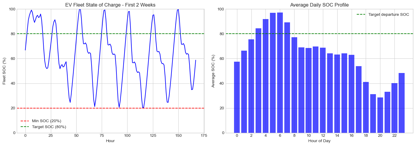
9. EV Impact on Grid#
[30]:
# Compare EV load with total system load
if len(ev_chargers) > 0 and len(n.links_t.p0) > 0:
    charger_cols = [c for c in n.links_t.p0.columns if c in ev_chargers.index]

    if charger_cols:
        # EV charging (net of V2G if present)
        ev_charging = n.links_t.p0[charger_cols].sum(axis=1) / 1000  # GW

        if len(v2g_links) > 0:
            v2g_cols = [c for c in n.links_t.p0.columns if c in v2g_links.index]
            if v2g_cols:
                v2g_discharge = n.links_t.p0[v2g_cols].sum(axis=1) / 1000  # GW
                net_ev_load = ev_charging - v2g_discharge
            else:
                net_ev_load = ev_charging
        else:
            net_ev_load = ev_charging

        # Total system load (from base electricity loads)
        # Base loads have carrier 'electricity' (not empty string)
        base_loads = n.loads[n.loads['carrier'] == 'electricity']
        base_cols = [c for c in n.loads_t.p_set.columns if c in base_loads.index]
        total_base_load = n.loads_t.p_set[base_cols].sum(axis=1) / 1000  # GW

        # Plot comparison
        fig, ax = plt.subplots(figsize=(14, 6))

        ax.fill_between(total_base_load.index, total_base_load.values,
                       alpha=0.5, label='Base Load', color='gray')
        ax.fill_between(net_ev_load.index, net_ev_load.values,
                       alpha=0.7, label='Net EV Load', color='green')

        ax.set_ylabel('Power (GW)')
        ax.set_xlabel('Time')
        ax.set_title('EV Impact on Total System Load')
        ax.legend()

        plt.tight_layout()
        plt.show()

        # Calculate EV share
        ev_share = net_ev_load.sum() / (total_base_load.sum() + net_ev_load.sum()) * 100
        print(f"\nEV Contribution to Total Load:")
        print(f"  EV share of total energy: {ev_share:.1f}%")
        print(f"  Peak coincidence factor: {net_ev_load.max() / ev_charging.max():.2f}")
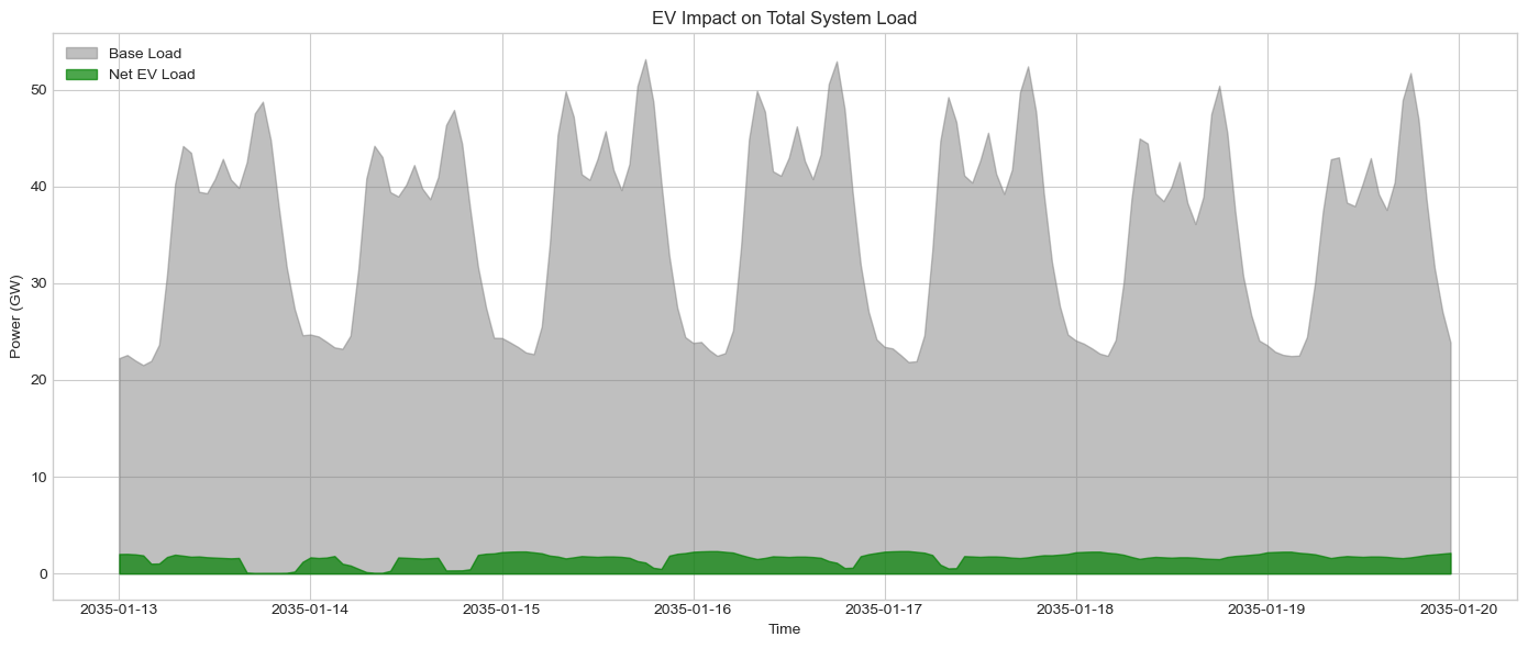
EV Contribution to Total Load:
  EV share of total energy: 4.3%
  Peak coincidence factor: 1.00
10. Configuration Reference#
EV flexibility is configured in config/defaults.yaml:
electric_vehicles:
  enabled: true
  tariff: "V2G"               # GO, INT, V2G, or MIXED

  # Flex share: Fraction of EVs with smart charging capability
  flex_share: 1.0              # 1.0 = all EVs, 0.2 = only 20%

  # Spatial allocation method
  allocation_method: "proportional"  # proportional, uniform, or urban_weighted

  # Fleet characteristics
  battery_capacity_kwh: 60.0   # Average EV battery size
  charge_efficiency: 0.90      # Grid-to-battery efficiency
  charger_power_kw: 7.0        # Home charger power

  # Availability profile
  use_traffic_data: true       # Use inverse of traffic for availability
  min_availability: 0.5        # Minimum plugged-in fraction during commute
  max_availability: 0.95       # Maximum plugged-in fraction overnight

  # V2G settings (when tariff: "V2G")
  v2g:
    use_fes_capacity: true     # Use FES Srg_BB005 V2G capacity
    discharge_efficiency: 0.90 # Battery-to-grid efficiency
    degradation_cost_per_mwh: 50.0  # Battery wear cost (£/MWh)

  # MIXED tariff shares (when tariff: "MIXED")
  mixed_tariff_shares:
    go_share: 0.5
    int_share: 0.3
    v2g_share: 0.2
Key Parameters:#
Parameter |
Description |
Typical Value |
|---|---|---|
|
Flexibility mode |
GO, INT, V2G, MIXED |
|
Fraction of EVs participating in flexibility |
0.1-1.0 |
|
How to distribute EVs geographically |
proportional |
|
Average EV battery size |
40-100 kWh |
|
Charging efficiency |
0.85-0.95 |
|
Home charger power |
3.5-22 kW |
|
Use FES V2G capacity projection |
true/false |
|
Battery cycling cost |
30-100 £/MWh |
|
Min plugged-in fraction (commute) |
0.4-0.6 |
|
Max plugged-in fraction (overnight) |
0.9-1.0 |
11. Advanced Features#
11.1 Spatial Allocation Methods#
PyPSA-GB provides three methods for allocating EV demand across network buses:
Method |
Description |
Use Case |
|---|---|---|
proportional |
Allocates based on existing demand |
Default - preserves demand patterns |
uniform |
Equal distribution across all buses |
Testing/sensitivity |
urban_weighted |
Concentrates EVs in high-demand areas |
Realistic urban concentration |
electric_vehicles:
  allocation_method: "proportional"  # or "uniform" or "urban_weighted"
The urban_weighted method uses a power function (exponent 2.0) to concentrate EVs in high-demand (urban) areas, reflecting the reality that EV adoption is higher in cities.
11.2 MIXED Tariff Mode#
The MIXED mode allows different EVs to use different tariff types at the same bus. For example:
50% on GO tariff (fixed window)
30% on INT tariff (smart charging)
20% on V2G tariff (bidirectional)
This reflects real-world heterogeneity where not all EV owners have the same charging infrastructure or willingness to participate in V2G.
electric_vehicles:
  tariff: "MIXED"
  mixed_tariff_shares:
    go_share: 0.5
    int_share: 0.3
    v2g_share: 0.2
The shares must sum to 1.0. MIXED mode creates separate Store and Link components for each tariff type at each bus.
11.4 EV Driving Profiles#
EV electricity demand follows traffic patterns with distinct peaks during commute times. PyPSA-GB uses a multi-modal synthetic profile with:
Morning peak: 08:00 (commute to work)
Midday activity: 10:00-16:00 (lunch, errands)
Evening peak: 18:00 (commute home)
This creates a realistic 2.8x peak-to-mean ratio, much more realistic than older single-peak profiles that concentrated all demand in a 4-hour window.
[32]:
# Visualize EV driving profile in detail
if len(ev_loads) > 0:
    driving_profile = n.loads_t.p_set[ev_loads.index].sum(axis=1) / 1000  # GW

    # Daily average pattern
    driving_by_hour = driving_profile.groupby(driving_profile.index.hour).mean()

    fig, axes = plt.subplots(2, 1, figsize=(14, 10))

    # Hourly bar chart with annotations
    bars = axes[0].bar(driving_by_hour.index, driving_by_hour.values, color='blue', alpha=0.7)
    axes[0].axhline(y=driving_by_hour.mean(), color='red', linestyle='--',
                    label=f'Mean: {driving_by_hour.mean():.2f} GW')

    # Highlight peak hours
    peak_hours = driving_by_hour.nlargest(2).index.tolist()
    for hour in peak_hours:
        bars[hour].set_color('red')
        bars[hour].set_alpha(0.8)

    axes[0].set_ylabel('Average Driving Demand (GW)')
    axes[0].set_xlabel('Hour of Day')
    axes[0].set_title('Average Daily EV Driving Profile')
    axes[0].set_xticks(range(0, 24, 1))
    axes[0].legend()
    axes[0].grid(True, alpha=0.3)

    # Add peak annotations
    for hour in peak_hours:
        axes[0].annotate(f'{driving_by_hour[hour]:.2f} GW\n(commute peak)',
                        xy=(hour, driving_by_hour[hour]),
                        xytext=(hour, driving_by_hour[hour] + 0.5),
                        ha='center', fontsize=9, color='red',
                        bbox=dict(boxstyle='round,pad=0.3', facecolor='yellow', alpha=0.7))

    # Full week time series
    week_data = driving_profile.iloc[:168]  # First week
    axes[1].plot(range(len(week_data)), week_data.values, linewidth=1.5, color='blue')
    axes[1].fill_between(range(len(week_data)), week_data.values, alpha=0.3, color='blue')
    axes[1].axhline(y=driving_profile.mean(), color='red', linestyle='--',
                   label=f'Mean: {driving_profile.mean():.2f} GW')

    # Mark weekdays
    for day in range(0, 168, 24):
        axes[1].axvline(x=day, color='gray', linestyle=':', alpha=0.5)
        day_name = ['Mon', 'Tue', 'Wed', 'Thu', 'Fri', 'Sat', 'Sun'][day//24]
        axes[1].text(day + 12, axes[1].get_ylim()[1] * 0.9, day_name,
                    ha='center', fontsize=9, color='gray')

    axes[1].set_ylabel('EV Driving Demand (GW)')
    axes[1].set_xlabel('Hour of Week')
    axes[1].set_title('EV Driving Profile - First Week')
    axes[1].legend()
    axes[1].grid(True, alpha=0.3)

    plt.tight_layout()
    plt.show()

    # Statistics
    peak_mean_ratio = driving_profile.max() / driving_profile.mean()
    print(f"\nDriving Profile Statistics:")
    print(f"  Peak: {driving_profile.max():.2f} GW at hour {driving_profile.idxmax().hour}:00")
    print(f"  Mean: {driving_profile.mean():.2f} GW")
    print(f"  Peak/Mean ratio: {peak_mean_ratio:.2f}x")
    print(f"  Peak hours: {[f'{h:02d}:00' for h in peak_hours]}")
else:
    print("No EV driving loads found")
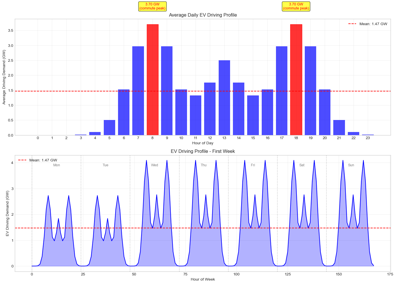
Driving Profile Statistics:
  Peak: 4.09 GW at hour 8:00
  Mean: 1.47 GW
  Peak/Mean ratio: 2.79x
  Peak hours: ['08:00', '18:00']
11.5 EV Components Architecture#
Understanding the PyPSA components created for EV flexibility:
Main Grid Bus (e.g., "ABCD1")
    │
    ├─ Load: "electric_vehicles" (dumb charging, if flex_share < 1.0)
    │
    └─ Link: "EV_charger_ABCD1_GO" (or INT/V2G)
            │ efficiency = 0.90 (charger efficiency)
            │ p_max_pu = availability profile (0.5-0.95)
            ↓
       EV Battery Bus: "ABCD1_ev_battery_GO"
            │
            ├─ Store: "EV_battery_ABCD1_GO"
            │       e_nom = battery capacity (MWh)
            │       e_min_pu = 0.2 (minimum 20% SOC)
            │       e_max_pu = 1.0 (full charge)
            │
            ├─ Load: "EV_driving_ABCD1_GO"
            │       p_set = driving demand profile
            │
            └─ Link: "V2G_ABCD1" (V2G mode only)
                    │ efficiency = 0.90
                    │ marginal_cost = 50 £/MWh (degradation)
                    ↓
               Back to Main Grid Bus
Key Observations:
Each tariff mode creates a separate EV battery bus
Store tracks state of charge over time
Charger Link limits charging based on availability
V2G adds reverse Link with degradation cost
MIXED mode creates multiple sets of components per bus
[33]:
# Examine component details at a sample bus

# Find a bus with EV components
if len(ev_stores) > 0:
    # Get a sample EV store and its bus
    sample_store = ev_stores.iloc[0]
    ev_bus = sample_store.name  # Store name is the bus name

    # Find the parent grid bus (EV bus ends with _ev_battery_...)
    # Extract grid bus name from EV bus
    grid_bus = ev_bus.split('_ev_battery')[0]

    print("=" * 70)
    print(f"EV COMPONENTS AT BUS: {grid_bus}")
    print("=" * 70)

    # Find all EV-related components at this bus

    # 1. Charger Link (grid → EV battery)
    charger_links = n.links[(n.links.bus0 == grid_bus) & (n.links.bus1.str.contains('ev_battery', na=False))]
    if len(charger_links) > 0:
        print(f"\n1. CHARGER LINK(S): {len(charger_links)}")
        for idx, link in charger_links.iterrows():
            print(f"   {idx}")
            print(f"     Carrier: {link['carrier']}")
            print(f"     Capacity: {link['p_nom']:.2f} MW")
            print(f"     Efficiency: {link['efficiency']:.2f}")
            if idx in n.links_t.p_max_pu.columns:
                avail = n.links_t.p_max_pu[idx]
                print(f"     Availability: {avail.min():.2f} - {avail.max():.2f}")

    # 2. EV Battery Store
    ev_stores_at_bus = n.stores[n.stores.index == ev_bus]
    if len(ev_stores_at_bus) > 0:
        print(f"\n2. BATTERY STORE(S): {len(ev_stores_at_bus)}")
        for idx, store in ev_stores_at_bus.iterrows():
            print(f"   {idx}")
            print(f"     Carrier: {store['carrier']}")
            print(f"     Capacity: {store['e_nom']:.2f} MWh")
            print(f"     Min SOC: {store.get('e_min_pu', 0)*100:.0f}%")
            print(f"     Max SOC: {store.get('e_max_pu', 1)*100:.0f}%")

    # 3. Driving Loads
    driving_loads_at_bus = n.loads[(n.loads.bus == ev_bus) & (n.loads.carrier == 'EV driving')]
    if len(driving_loads_at_bus) > 0:
        print(f"\n3. DRIVING LOAD(S): {len(driving_loads_at_bus)}")
        for idx, load in driving_loads_at_bus.iterrows():
            total_demand = n.loads_t.p_set[idx].sum() if idx in n.loads_t.p_set.columns else 0
            print(f"   {idx}")
            print(f"     Carrier: {load['carrier']}")
            print(f"     Total weekly demand: {total_demand:.1f} MWh")
            print(f"     Peak demand: {n.loads_t.p_set[idx].max():.2f} MW")

    # 4. V2G Link (if present)
    v2g_at_bus = n.links[(n.links.bus0 == ev_bus) & (n.links.bus1 == grid_bus) & (n.links.carrier == 'V2G')]
    if len(v2g_at_bus) > 0:
        print(f"\n4. V2G LINK(S): {len(v2g_at_bus)}")
        for idx, link in v2g_at_bus.iterrows():
            print(f"   {idx}")
            print(f"     Capacity: {link['p_nom']:.2f} MW")
            print(f"     Efficiency: {link['efficiency']:.2f}")
            print(f"     Degradation cost: £{link.get('marginal_cost', 0):.2f}/MWh")

    # 5. Dumb EV loads (if flex_share < 1.0)
    dumb_loads_at_bus = n.loads[(n.loads.bus == grid_bus) & (n.loads.carrier == 'electric_vehicles')]
    if len(dumb_loads_at_bus) > 0:
        print(f"\n5. DUMB EV LOAD(S): {len(dumb_loads_at_bus)}")
        for idx, load in dumb_loads_at_bus.iterrows():
            total_demand = n.loads_t.p_set[idx].sum() if idx in n.loads_t.p_set.columns else 0
            print(f"   {idx}")
            print(f"     Total weekly demand: {total_demand:.1f} MWh")
            print(f"     (This is the non-flexible portion)")

    print("\n" + "=" * 70)
else:
    print("No EV stores found in network")
======================================================================
EV COMPONENTS AT BUS: CLAC1Q EV fleet battery GO
======================================================================

2. BATTERY STORE(S): 1
   CLAC1Q EV fleet battery GO
     Carrier: EV battery
     Capacity: 0.96 MWh
     Min SOC: 20%
     Max SOC: 100%

======================================================================
12. Comparing Scenarios & Understanding Value#
To understand the value of EV flexibility, you can compare scenarios with different tariff modes:
Scenario |
Description |
Expected Results |
|---|---|---|
No flex |
EVs as dumb loads |
High evening peak, no system services |
GO |
Fixed night window |
Peak shifted but not optimized |
INT |
Smart charging |
Optimized charging timing, lower costs |
V2G |
Bidirectional |
Additional grid services, highest value |
Value of flexibility comes from:
Peak shaving: Reducing evening demand peaks (£100-200/MWh avoided)
Renewable integration: Charging when wind/solar abundant (£30-50/MWh)
Grid services (V2G): Providing balancing during stress (£100-300/MWh)
Transmission relief: Distributing load temporally reduces network congestion
Trade-offs:
GO: Simple but inflexible (fixed window may not align with cheap power)
INT: Good balance of value and simplicity
V2G: Highest value but requires bidirectional chargers + degradation costs
MIXED: Most realistic but more complex to model
13. Summary & Key Takeaways#
Key Takeaways:#
EV flexibility provides significant grid value through:
Peak demand reduction (smart charging shifts load overnight)
Grid balancing services (V2G discharges during stress periods)
Renewable integration (charge when wind/solar abundant)
Network congestion relief (temporal load distribution)
Four tariff modes offer different flexibility levels:
GO: Simple time shift to fixed 4-hour window (00:00-04:00)
INT: Full optimization of charging timing
V2G: Bidirectional including grid export
MIXED: Heterogeneous fleet with different tariff types per bus
Spatial allocation methods control geographic distribution:
proportional: Preserves existing demand patterns (default)
uniform: Equal distribution for testing
urban_weighted: Concentrates EVs in high-demand (urban) areas
flex_share is the key parameter (default 0.2 = 20%):
Controls demand split: 20% flexible, 80% dumb
Dumb loads merge into base ‘electricity’ during clustering
Flexible portion gets optimizable Store + Link components
Hardware capacities from FES building blocks:
V2G: FES Srg_BB005 (~17.9 GW for HT 2035)
Smart charging: FES Srg_BB007a
Scaled by: flex_share × MIXED mode tariff shares
Battery degradation cost (£50/MWh) limits V2G cycling
Multi-modal driving profile reflects realistic traffic:
Morning peak (08:00) + Evening peak (18:00)
Midday activity for errands
2.8x peak-to-mean ratio (much better than old 5.5x single-peak)
PyPSA components for EV flexibility:
Store (EV battery): Tracks SOC, enforces capacity limits
Link (EV charger): Connects grid to battery with efficiency + availability
Link (V2G): Connects battery back to grid for discharge
Load (EV driving): Fixed demand for vehicle operation
Load (dumb EVs): Non-flexible portion, merged into ‘electricity’ during clustering
Further Exploration#
Try different
flex_sharevalues (0.2, 0.5, 1.0) to see adoption rate impactsCompare GO vs INT vs V2G costs and load profiles
Examine V2G dispatch during different weather/demand conditions
Analyze network congestion with/without EV smart charging
Test sensitivity to
degradation_cost_per_mwhin V2G scenarios