Storage Systems#
This tutorial covers electricity storage modeling in PyPSA-GB, including batteries and pumped hydro.
What You’ll Learn#
Storage capacity and parameters
State of charge dynamics
Charging and discharging patterns
Storage arbitrage and value
Comparing storage technologies
1. Setup#
[1]:
import pypsa
import pandas as pd
import numpy as np
import matplotlib.pyplot as plt
import warnings
import folium
from pyproj import Transformer

warnings.filterwarnings('ignore')
plt.style.use('seaborn-v0_8-whitegrid')
plt.rcParams['figure.figsize'] = [12, 6]
plt.rcParams['figure.dpi'] = 100

colors = {
    'battery': '#9C27B0', 'pumped_hydro': '#3F51B5', 'storage': '#673AB7',
    'charging': '#E91E63', 'discharging': '#4CAF50'
}

print(f"PyPSA version: {pypsa.__version__}")
PyPSA version: 1.0.7
2. Load Network#
[2]:
# Load a network with storage
n = pypsa.Network("../../../resources/network/HT35_clustered_solved.nc")

print(f"Network loaded")
print(f"  Snapshots: {len(n.snapshots)}")
print(f"  Storage Units: {len(n.storage_units)}")
INFO:pypsa.network.io:Imported network 'HT35_clustered (Clustered)' has buses, carriers, generators, lines, links, loads, storage_units, stores, sub_networks
Network loaded
  Snapshots: 168
  Storage Units: 784
3. Storage Capacity Overview#
[3]:
# Storage capacity summary
storage = n.storage_units.copy()

print(f"Total storage units: {len(storage)}")

# Capacity by carrier
capacity = storage.groupby('carrier').agg({
    'p_nom': 'sum',       # Power capacity (MW)
    'max_hours': 'mean'   # Average duration (hours)
})

capacity['p_nom_GW'] = capacity['p_nom'] / 1000
capacity['energy_GWh'] = capacity['p_nom_GW'] * capacity['max_hours']

print("\nStorage Capacity:")
for carrier in capacity.index:
    print(f"\n{carrier}:")
    print(f"  Power: {capacity.loc[carrier, 'p_nom_GW']:.2f} GW")
    print(f"  Duration: {capacity.loc[carrier, 'max_hours']:.1f} hours")
    print(f"  Energy: {capacity.loc[carrier, 'energy_GWh']:.2f} GWh")
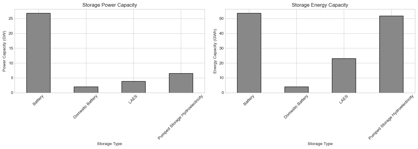
Total storage units: 784

Storage Capacity:

Battery:
  Power: 26.77 GW
  Duration: 2.0 hours
  Energy: 53.54 GWh

Domestic Battery:
  Power: 1.99 GW
  Duration: 2.0 hours
  Energy: 3.98 GWh

LAES:
  Power: 3.85 GW
  Duration: 6.0 hours
  Energy: 23.11 GWh

Pumped Storage Hydroelectricity:
  Power: 6.49 GW
  Duration: 8.0 hours
  Energy: 51.88 GWh
[4]:
# Capacity bar chart
fig, axes = plt.subplots(1, 2, figsize=(14, 5))

# Power capacity
ax1 = axes[0]
bar_colors = [colors.get(c, '#888888') for c in capacity.index]
capacity['p_nom_GW'].plot(kind='bar', ax=ax1, color=bar_colors, edgecolor='black')
ax1.set_ylabel('Power Capacity (GW)')
ax1.set_xlabel('Storage Type')
ax1.set_title('Storage Power Capacity')
ax1.tick_params(axis='x', rotation=45)

# Energy capacity
ax2 = axes[1]
capacity['energy_GWh'].plot(kind='bar', ax=ax2, color=bar_colors, edgecolor='black')
ax2.set_ylabel('Energy Capacity (GWh)')
ax2.set_xlabel('Storage Type')
ax2.set_title('Storage Energy Capacity')
ax2.tick_params(axis='x', rotation=45)

plt.tight_layout()
plt.show()
4. Storage Parameters#
[5]:
# Key storage parameters
params = storage.groupby('carrier').agg({
    'efficiency_store': 'mean',     # Charging efficiency
    'efficiency_dispatch': 'mean',  # Discharging efficiency
    'standing_loss': 'mean',        # Self-discharge rate
    'marginal_cost': 'mean',        # Dispatch cost
    'cyclic_state_of_charge': 'first'  # Cyclic constraint
})

params['round_trip_efficiency'] = params['efficiency_store'] * params['efficiency_dispatch'] * 100

print("Storage Parameters:")
for carrier in params.index:
    print(f"\n{carrier}:")
    print(f"  Charging Efficiency: {params.loc[carrier, 'efficiency_store']*100:.1f}%")
    print(f"  Discharging Efficiency: {params.loc[carrier, 'efficiency_dispatch']*100:.1f}%")
    print(f"  Round-Trip Efficiency: {params.loc[carrier, 'round_trip_efficiency']:.1f}%")
    print(f"  Standing Loss: {params.loc[carrier, 'standing_loss']*100:.3f}%/hour")
Storage Parameters:

Battery:
  Charging Efficiency: 92.0%
  Discharging Efficiency: 92.0%
  Round-Trip Efficiency: 84.6%
  Standing Loss: 0.100%/hour

Domestic Battery:
  Charging Efficiency: 92.0%
  Discharging Efficiency: 92.0%
  Round-Trip Efficiency: 84.6%
  Standing Loss: 0.100%/hour

LAES:
  Charging Efficiency: 60.0%
  Discharging Efficiency: 60.0%
  Round-Trip Efficiency: 36.0%
  Standing Loss: 0.100%/hour

Pumped Storage Hydroelectricity:
  Charging Efficiency: 87.0%
  Discharging Efficiency: 87.0%
  Round-Trip Efficiency: 75.7%
  Standing Loss: 0.100%/hour
5. State of Charge Analysis#
[6]:
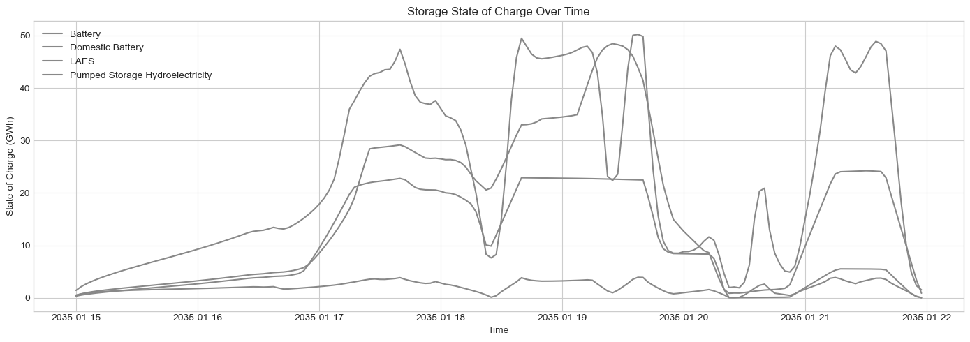
# State of charge time series
soc = n.storage_units_t.state_of_charge

print(f"State of Charge data shape: {soc.shape}")

# Aggregate by carrier
soc_by_carrier = soc.groupby(n.storage_units.carrier, axis=1).sum() / 1000  # GWh

print("\nState of Charge Statistics (GWh):")
print(soc_by_carrier.describe().round(2))
State of Charge data shape: (168, 784)

State of Charge Statistics (GWh):
carrier  Battery  Domestic Battery    LAES  Pumped Storage Hydroelectricity
count     168.00            168.00  168.00                           168.00
mean       23.24              2.11   10.02                            16.64
std        16.46              1.01    8.75                            13.92
min         1.44              0.02    0.06                             0.48
25%         8.67              1.37    2.39                             3.45
50%        16.40              1.99    5.53                            13.75
75%        41.05              3.06   20.57                            26.64
max        50.22              3.93   22.91                            48.46
[7]:
# State of charge time series plot
fig, ax = plt.subplots(figsize=(14, 5))

for col in soc_by_carrier.columns:
    ax.plot(soc_by_carrier.index, soc_by_carrier[col],
            color=colors.get(col, '#888888'), linewidth=1.5, label=col)

ax.set_ylabel('State of Charge (GWh)')
ax.set_xlabel('Time')
ax.set_title('Storage State of Charge Over Time')
ax.legend()

plt.tight_layout()
plt.show()
[8]:
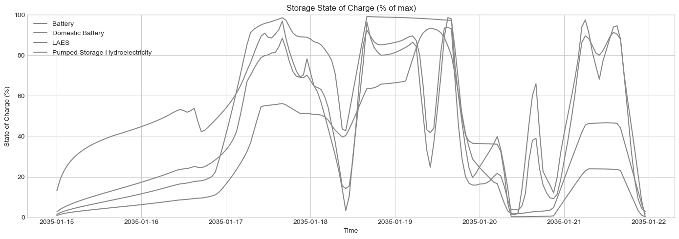
# SOC percentage (normalized)
fig, ax = plt.subplots(figsize=(14, 5))

for carrier in soc_by_carrier.columns:
    carrier_storage = n.storage_units[n.storage_units.carrier == carrier]
    max_energy = (carrier_storage['p_nom'] * carrier_storage['max_hours']).sum() / 1000
    soc_pct = soc_by_carrier[carrier] / max_energy * 100

    ax.plot(soc_pct.index, soc_pct.values,
            color=colors.get(carrier, '#888888'), linewidth=1.5, label=carrier)

ax.set_ylabel('State of Charge (%)')
ax.set_xlabel('Time')
ax.set_title('Storage State of Charge (% of max)')
ax.legend()
ax.set_ylim(0, 100)

plt.tight_layout()
plt.show()
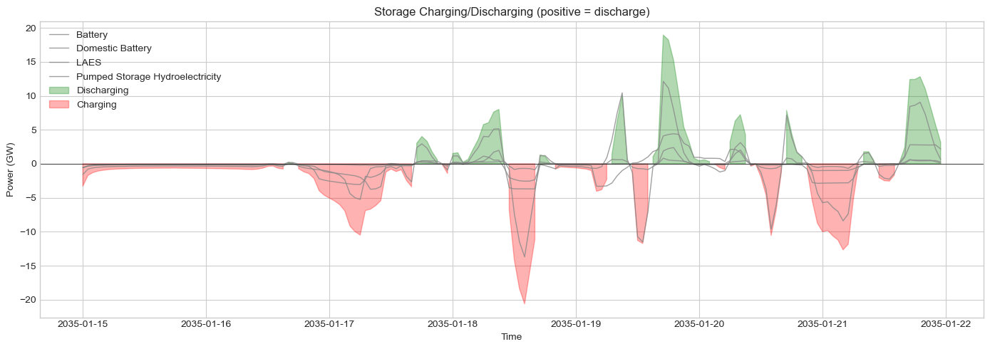
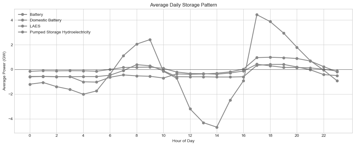
6. Charging and Discharging Patterns#
[9]:
# Power dispatch (positive = discharge, negative = charge)
power = n.storage_units_t.p

# Aggregate by carrier
power_by_carrier = power.groupby(n.storage_units.carrier, axis=1).sum() / 1000  # GW

print("Storage Power Statistics (GW):")
print(power_by_carrier.describe().round(2))
Storage Power Statistics (GW):
carrier  Battery  Domestic Battery    LAES  Pumped Storage Hydroelectricity
count     168.00            168.00  168.00                           168.00
mean       -0.31             -0.03   -0.28                            -0.18
std         3.79              0.33    1.06                             1.51
min       -13.70             -0.87   -3.70                            -3.75
25%        -0.99             -0.15   -0.21                            -0.34
50%        -0.34             -0.06   -0.03                            -0.13
75%         0.47              0.17    0.00                             0.08
max        12.13              0.84    2.39                             4.42
[10]:
# Power dispatch plot
fig, ax = plt.subplots(figsize=(14, 5))

for col in power_by_carrier.columns:
    ax.plot(power_by_carrier.index, power_by_carrier[col],
            color=colors.get(col, '#888888'), linewidth=1, label=col, alpha=0.8)

ax.axhline(y=0, color='black', linestyle='-', linewidth=0.5)
ax.fill_between(power_by_carrier.index, power_by_carrier.sum(axis=1),
               where=power_by_carrier.sum(axis=1) > 0, alpha=0.3, color='green', label='Discharging')
ax.fill_between(power_by_carrier.index, power_by_carrier.sum(axis=1),
               where=power_by_carrier.sum(axis=1) < 0, alpha=0.3, color='red', label='Charging')

ax.set_ylabel('Power (GW)')
ax.set_xlabel('Time')
ax.set_title('Storage Charging/Discharging (positive = discharge)')
ax.legend()

plt.tight_layout()
plt.show()
[11]:
# Daily pattern
power_hourly = power_by_carrier.groupby(power_by_carrier.index.hour).mean()

fig, ax = plt.subplots(figsize=(12, 5))

for col in power_hourly.columns:
    ax.plot(power_hourly.index, power_hourly[col],
            color=colors.get(col, '#888888'), linewidth=2, marker='o', label=col)

ax.axhline(y=0, color='black', linestyle='-', linewidth=0.5)
ax.set_xlabel('Hour of Day')
ax.set_ylabel('Average Power (GW)')
ax.set_title('Average Daily Storage Pattern')
ax.set_xticks(range(0, 24, 2))
ax.legend()

plt.tight_layout()
plt.show()
7. Storage Utilization#
[12]:
# Calculate utilization metrics
utilization = []

for carrier in power_by_carrier.columns:
    carrier_storage = n.storage_units[n.storage_units.carrier == carrier]
    total_capacity = carrier_storage['p_nom'].sum() / 1000  # GW

    if total_capacity > 0:
        # Total energy discharged
        discharged = power_by_carrier[carrier][power_by_carrier[carrier] > 0].sum()  # GWh
        charged = -power_by_carrier[carrier][power_by_carrier[carrier] < 0].sum()  # GWh

        # Capacity factor based on discharge
        hours = len(n.snapshots)
        cf = discharged / (total_capacity * hours) * 100

        # Cycles (discharge energy / energy capacity)
        energy_capacity = (carrier_storage['p_nom'] * carrier_storage['max_hours']).sum() / 1000
        cycles = discharged / energy_capacity if energy_capacity > 0 else 0

        utilization.append({
            'Carrier': carrier,
            'Power (GW)': total_capacity,
            'Discharged (GWh)': discharged,
            'Charged (GWh)': charged,
            'Capacity Factor (%)': cf,
            'Cycles': cycles
        })

util_df = pd.DataFrame(utilization).set_index('Carrier')
print("Storage Utilization:")
util_df.round(2)
Storage Utilization:
[12]:
| Power (GW) | Discharged (GWh) | Charged (GWh) | Capacity Factor (%) | Cycles | |
|---|---|---|---|---|---|
| Carrier | |||||
| Battery | 26.77 | 165.88 | 218.67 | 3.69 | 3.10 |
| Domestic Battery | 1.99 | 17.40 | 23.21 | 5.20 | 4.37 |
| LAES | 3.85 | 23.68 | 70.98 | 3.66 | 1.02 |
| Pumped Storage Hydroelectricity | 6.49 | 66.38 | 96.71 | 6.09 | 1.28 |
8. Arbitrage Value#
[13]:
# Calculate arbitrage value using marginal prices
if 'marginal_price' in n.buses_t and len(n.buses_t.marginal_price.columns) > 0:
    lmps = n.buses_t.marginal_price

    # Revenue from arbitrage = discharge × price - charge × price
    arbitrage = []

    for carrier in power_by_carrier.columns:
        carrier_storage = n.storage_units[n.storage_units.carrier == carrier]

        total_revenue = 0
        total_cost = 0

        for unit in carrier_storage.index:
            if unit in power.columns:
                bus = n.storage_units.loc[unit, 'bus']
                if bus in lmps.columns:
                    p = power[unit]
                    price = lmps[bus]

                    # Discharge revenue
                    discharge = p[p > 0]
                    revenue = (discharge * price[p > 0]).sum()

                    # Charge cost
                    charge = -p[p < 0]
                    cost = (charge * price[p < 0]).sum()

                    total_revenue += revenue
                    total_cost += cost

        arbitrage.append({
            'Carrier': carrier,
            'Revenue (£M)': total_revenue / 1e6,
            'Cost (£M)': total_cost / 1e6,
            'Profit (£M)': (total_revenue - total_cost) / 1e6
        })

    arb_df = pd.DataFrame(arbitrage).set_index('Carrier')
    print("Storage Arbitrage Value:")
    print(arb_df.round(2))
else:
    print("Marginal prices not available - re-solve with keep_shadowprices=True")
Storage Arbitrage Value:
                                 Revenue (£M)  Cost (£M)  Profit (£M)
Carrier
Battery                                  3.90       1.64         2.26
Domestic Battery                         0.39       0.21         0.18
LAES                                     0.65       0.20         0.44
Pumped Storage Hydroelectricity          1.11       0.28         0.83
[14]:
# Average charge/discharge prices
if 'marginal_price' in n.buses_t and len(n.buses_t.marginal_price.columns) > 0:
    avg_prices = []

    for carrier in power_by_carrier.columns:
        carrier_storage = n.storage_units[n.storage_units.carrier == carrier]

        all_discharge_prices = []
        all_charge_prices = []

        for unit in carrier_storage.index:
            if unit in power.columns:
                bus = n.storage_units.loc[unit, 'bus']
                if bus in lmps.columns:
                    p = power[unit]
                    price = lmps[bus]

                    all_discharge_prices.extend(price[p > 0].values)
                    all_charge_prices.extend(price[p < 0].values)

        avg_prices.append({
            'Carrier': carrier,
            'Avg Discharge Price (£/MWh)': np.mean(all_discharge_prices) if all_discharge_prices else 0,
            'Avg Charge Price (£/MWh)': np.mean(all_charge_prices) if all_charge_prices else 0,
            'Spread (£/MWh)': np.mean(all_discharge_prices) - np.mean(all_charge_prices) if all_discharge_prices and all_charge_prices else 0
        })

    price_df = pd.DataFrame(avg_prices).set_index('Carrier')
    print("Average Charge/Discharge Prices:")
    print(price_df.round(2))
Average Charge/Discharge Prices:
                                 Avg Discharge Price (£/MWh)  \
Carrier
Battery                                                17.02
Domestic Battery                                       15.67
LAES                                                   21.56
Pumped Storage Hydroelectricity                        18.77

                                 Avg Charge Price (£/MWh)  Spread (£/MWh)
Carrier
Battery                                              6.49           10.54
Domestic Battery                                     5.17           10.50
LAES                                                 6.08           15.47
Pumped Storage Hydroelectricity                      6.40           12.37
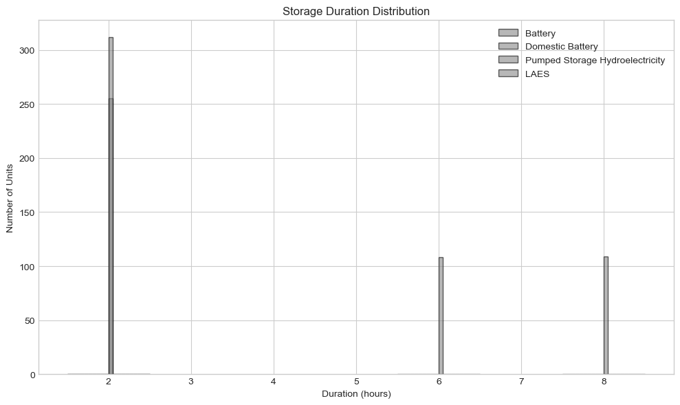
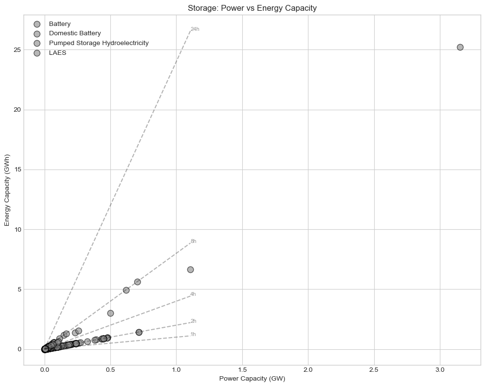
9. Comparing Storage Technologies#
[15]:
# Duration distribution
fig, ax = plt.subplots(figsize=(10, 6))

for carrier in storage['carrier'].unique():
    carrier_data = storage[storage.carrier == carrier]['max_hours']
    ax.hist(carrier_data, bins=20, alpha=0.6,
           color=colors.get(carrier, '#888888'), label=carrier, edgecolor='black')

ax.set_xlabel('Duration (hours)')
ax.set_ylabel('Number of Units')
ax.set_title('Storage Duration Distribution')
ax.legend()

plt.tight_layout()
plt.show()
[16]:
# Power vs Energy capacity scatter
fig, ax = plt.subplots(figsize=(10, 8))

for carrier in storage['carrier'].unique():
    carrier_data = storage[storage.carrier == carrier]
    power_gw = carrier_data['p_nom'] / 1000
    energy_gwh = power_gw * carrier_data['max_hours']

    ax.scatter(power_gw, energy_gwh, s=80, alpha=0.6,
              color=colors.get(carrier, '#888888'), label=carrier, edgecolors='black')

# Reference lines for duration
for hours in [1, 2, 4, 8, 24]:
    x = np.linspace(0, power_gw.max(), 100)
    ax.plot(x, x * hours, 'k--', alpha=0.3)
    ax.annotate(f'{hours}h', xy=(x[-1], x[-1]*hours), fontsize=8, alpha=0.5)

ax.set_xlabel('Power Capacity (GW)')
ax.set_ylabel('Energy Capacity (GWh)')
ax.set_title('Storage: Power vs Energy Capacity')
ax.legend()

plt.tight_layout()
plt.show()
10. Geographic Distribution#
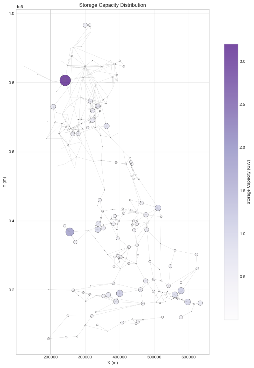
[17]:
# Storage capacity by bus
storage_by_bus = storage.groupby('bus')['p_nom'].sum() / 1000  # GW

fig, ax = plt.subplots(figsize=(10, 12))

# Get bus coordinates
bus_x = n.buses.loc[storage_by_bus.index, 'x']
bus_y = n.buses.loc[storage_by_bus.index, 'y']

# Size proportional to capacity
sizes = storage_by_bus * 200  # Scale for visibility

scatter = ax.scatter(bus_x, bus_y, s=sizes, c=storage_by_bus,
                    cmap='Purples', alpha=0.7, edgecolors='black', linewidth=0.5)

# Plot lines for context
for line in n.lines.index:
    bus0, bus1 = n.lines.loc[line, ['bus0', 'bus1']]
    if bus0 in n.buses.index and bus1 in n.buses.index:
        ax.plot([n.buses.loc[bus0, 'x'], n.buses.loc[bus1, 'x']],
               [n.buses.loc[bus0, 'y'], n.buses.loc[bus1, 'y']],
               color='gray', linewidth=0.3, alpha=0.5)

plt.colorbar(scatter, label='Storage Capacity (GW)', shrink=0.8)
ax.set_xlabel('X (m)')
ax.set_ylabel('Y (m)')
ax.set_title('Storage Capacity Distribution')
ax.set_aspect('equal')

plt.tight_layout()
plt.show()