Demand Side Response#
This tutorial demonstrates how PyPSA-GB models domestic Demand Side Response (DSR) - households reducing electricity consumption during peak periods in exchange for incentive payments.
DSR programs like National Grid ESO’s “Saving Sessions” provide crucial flexibility during winter peak demand by:
Reducing demand during critical 2-hour windows (typically 17:00-19:00)
Helping avoid blackouts and expensive peaker plants
Providing households with bill savings (£3-10/event)
The HT35_flex scenario includes 1,500 MW of domestic DSR capacity, representing household participation in demand response events.
What You’ll Learn#
DSR configuration modes (regular, winter, both)
Event scheduling patterns and frequency
DSR dispatch behavior and system value
Comparison with other flexibility mechanisms (EV, batteries)
Configuration parameters and capacity sizing
1. Setup#
[1]:
import pypsa
import pandas as pd
import numpy as np
import matplotlib.pyplot as plt
import yaml
import warnings

warnings.filterwarnings('ignore')
plt.style.use('seaborn-v0_8-whitegrid')
plt.rcParams['figure.figsize'] = [14, 6]
plt.rcParams['figure.dpi'] = 100

print(f"PyPSA version: {pypsa.__version__}")
PyPSA version: 1.0.7
2. Load Network with DSR#
The HT35_flex scenario includes event-based demand flexibility representing domestic DSR participation.
[2]:
# Load solved network with DSR enabled
n = pypsa.Network("../../../resources/network/HT30_event_response_solved.nc")

print("Network loaded")
print(f"  Buses: {len(n.buses)}")
print(f"  Generators: {len(n.generators)}")
print(f"  Period: {n.snapshots[0]} to {n.snapshots[-1]}")
print(f"  Snapshots: {len(n.snapshots)}")
INFO:pypsa.network.io:Imported network 'HT30_event_response (Clustered)' has buses, carriers, generators, lines, links, loads, storage_units, stores, sub_networks
Network loaded
  Buses: 20
  Generators: 161
  Period: 2030-02-21 00:00:00 to 2030-03-07 23:00:00
  Snapshots: 360
3. DSR Configuration#
Let’s examine how DSR is configured in the HT35_flex scenario.
[3]:
# Load configuration
with open("../../../config/defaults.yaml") as f:
    defaults = yaml.safe_load(f)

with open("../../../config/scenarios.yaml") as f:
    scenarios = yaml.safe_load(f)

# Get DSR configuration
dsr_defaults = defaults.get('demand_flexibility', {}).get('event_response', {})
scenario_dsr = scenarios.get('HT35_flex', {}).get('demand_flexibility', {}).get('event_response', {})

# Effective configuration (scenario overrides defaults)
eff_enabled = scenario_dsr.get('enabled', dsr_defaults.get('enabled', False))
eff_mode = scenario_dsr.get('mode', dsr_defaults.get('mode', 'regular'))
eff_capacity = scenario_dsr.get('dsr_capacity_mw', dsr_defaults.get('dsr_capacity_mw', None))
eff_window = scenario_dsr.get('event_window', dsr_defaults.get('event_window', ['17:00', '19:00']))
eff_winter_months = dsr_defaults.get('winter_months', [10, 11, 12, 1, 2, 3])

print("=" * 70)
print("HT35_FLEX DSR CONFIGURATION")
print("=" * 70)

print(f"\nENABLED: {eff_enabled}")

print(f"\nMODE: '{eff_mode}'")
if eff_mode == 'regular':
    print("  → 2 events per week throughout the year")
elif eff_mode == 'winter':
    print(f"  → 5 events per week during winter months {eff_winter_months}")
elif eff_mode == 'both':
    print(f"  → 2 events/week year-round + 5 events/week in winter {eff_winter_months}")

print(f"\nCAPACITY:")
if eff_capacity:
    print(f"  dsr_capacity_mw = {eff_capacity} MW (user-defined)")
else:
    part_rate = dsr_defaults.get('participation_rate', 0.33)
    max_red = dsr_defaults.get('max_reduction_fraction', 0.10)
    print(f"  Calculated from: participation_rate ({part_rate}) × max_reduction ({max_red})")

print(f"\nEVENT WINDOW:")
print(f"  {eff_window[0]} - {eff_window[1]} (peak demand period)")

print(f"\nWINTER MONTHS (for 'winter' or 'both' modes):")
month_names = ['Jan', 'Feb', 'Mar', 'Apr', 'May', 'Jun',
               'Jul', 'Aug', 'Sep', 'Oct', 'Nov', 'Dec']
winter_names = [month_names[m-1] for m in eff_winter_months]
print(f"  {', '.join(winter_names)}")

print("\n" + "=" * 70)
======================================================================
HT35_FLEX DSR CONFIGURATION
======================================================================

ENABLED: True

MODE: 'both'
  → 2 events/week year-round + 5 events/week in winter [10, 11, 12, 1, 2, 3]

CAPACITY:
  Calculated from: participation_rate (0.33) × max_reduction (0.1)

EVENT WINDOW:
  17:00 - 19:00 (peak demand period)

WINTER MONTHS (for 'winter' or 'both' modes):
  Oct, Nov, Dec, Jan, Feb, Mar

======================================================================
4. DSR Components in PyPSA#
DSR is modeled as Generator components with:
p_nom: Maximum demand reduction capacity (MW)
p_max_pu: Time-varying availability (0 or 1, only during events)
carrier: ‘demand response’
marginal_cost: High cost (£500/MWh) = only dispatch when needed
These generators represent households reducing consumption, which appears as “negative demand” or “generation” in the model.
[4]:
# Find DSR generators
dsr_gens = n.generators[n.generators.carrier == 'demand response']

print(f"DSR Generators: {len(dsr_gens)}")
print(f"Total DSR Capacity: {dsr_gens.p_nom.sum():.1f} MW")
print(f"Average per bus: {dsr_gens.p_nom.mean():.2f} MW")
print(f"Marginal cost: £{dsr_gens.marginal_cost.iloc[0]:.0f}/MWh (incentive payment)")

# Show sample DSR generators
print("\nSample DSR Generators:")
print(dsr_gens[['bus', 'carrier', 'p_nom', 'marginal_cost']].head(10))
DSR Generators: 11
Total DSR Capacity: 1483.2 MW
Average per bus: 134.84 MW
Marginal cost: £40/MWh (incentive payment)

Sample DSR Generators:
                                     bus          carrier       p_nom  \
name
ABHA11 demand response         cluster_5  demand response    8.167500
ABNE3- demand response__agg80  cluster_2  demand response   93.976345
ABTH11 demand response__agg26  cluster_5  demand response  193.985896
ALNE3J demand response__agg17  cluster_8  demand response    9.925903
AMEM11 demand response__agg56  cluster_3  demand response  464.719781
ARBR3- demand response__agg28  cluster_0  demand response   24.772280
BERW3- demand response__agg19  cluster_6  demand response   48.911278
BESW11 demand response__agg25  cluster_1  demand response  245.879089
BIRK11 demand response__agg25  cluster_9  demand response  212.920884
BRAW11 demand response__agg27  cluster_4  demand response  178.110098

                               marginal_cost
name
ABHA11 demand response                  40.0
ABNE3- demand response__agg80           40.0
ABTH11 demand response__agg26           40.0
ALNE3J demand response__agg17           40.0
AMEM11 demand response__agg56           40.0
ARBR3- demand response__agg28           40.0
BERW3- demand response__agg19           40.0
BESW11 demand response__agg25           40.0
BIRK11 demand response__agg25           40.0
BRAW11 demand response__agg27           40.0
5. DSR Dispatch Analysis#
Now let’s analyze when and how much DSR was actually dispatched by the optimizer.
[6]:
# Get DSR dispatch (actual demand reduction)
if len(dsr_gens) > 0 and len(n.generators_t.p) > 0:
    dsr_cols = [c for c in n.generators_t.p.columns if c in dsr_gens.index]

    if dsr_cols:
        # Total DSR dispatch across all buses
        total_dsr = n.generators_t.p[dsr_cols].sum(axis=1) / 1000  # GW

        print("=" * 70)
        print("DSR DISPATCH SUMMARY")
        print("=" * 70)

        print(f"\nCapacity vs Utilization:")
        print(f"  Total DSR capacity: {dsr_gens.p_nom.sum():.1f} MW")
        print(f"  Peak dispatch: {total_dsr.max():.2f} GW")
        print(f"  Peak utilization: {total_dsr.max() / (dsr_gens.p_nom.sum()/1000) * 100:.1f}%")

        print(f"\nEnergy Delivered:")
        print(f"  Total DSR energy: {total_dsr.sum():.1f} GWh")
        print(f"  Hours with DSR > 0: {(total_dsr > 0.001).sum()}")
        print(f"  Average during events: {total_dsr[total_dsr > 0.001].mean():.2f} GW")

        # Plot dispatch time series
        fig, axes = plt.subplots(2, 1, figsize=(14, 8), sharex=False)

        # Full time series
        axes[0].fill_between(total_dsr.index, total_dsr.values,
                            alpha=0.6, color='orange', label='DSR Dispatch')
        axes[0].axhline(y=dsr_gens.p_nom.sum()/1000, color='red', linestyle='--',
                       label=f'Total Capacity: {dsr_gens.p_nom.sum()/1000:.2f} GW')
        axes[0].set_ylabel('DSR Dispatch (GW)')
        axes[0].set_xlabel('Time')
        axes[0].set_title('Demand Side Response Dispatch Over Time')
        axes[0].legend()
        axes[0].grid(True, alpha=0.3)

        # Average by hour of day
        dsr_by_hour = total_dsr.groupby(total_dsr.index.hour).mean()

        bars = axes[1].bar(dsr_by_hour.index, dsr_by_hour.values,
                          color='orange', alpha=0.7)

        # Highlight event window
        window_start = int(eff_window[0].split(':')[0])
        window_end = int(eff_window[1].split(':')[0])
        for hour in range(window_start, window_end):
            if hour < len(bars):
                bars[hour].set_color('red')
                bars[hour].set_alpha(0.8)

        axes[1].set_ylabel('Average DSR (GW)')
        axes[1].set_xlabel('Hour of Day')
        axes[1].set_title(f'DSR Dispatch by Hour (Event Window: {eff_window[0]}-{eff_window[1]})')
        axes[1].set_xticks(range(0, 24, 1))
        axes[1].grid(True, alpha=0.3)

        # Add annotation for event window
        axes[1].axvspan(window_start, window_end, alpha=0.2, color='red',
                       label='Event Window')
        axes[1].legend()

        plt.tight_layout()
        plt.show()

        print("\n" + "=" * 70)
    else:
        print("No DSR dispatch data found")
else:
    print("No DSR generators found")
======================================================================
DSR DISPATCH SUMMARY
======================================================================

Capacity vs Utilization:
  Total DSR capacity: 1483.2 MW
  Peak dispatch: 1.48 GW
  Peak utilization: 100.0%

Energy Delivered:
  Total DSR energy: 3.0 GWh
  Hours with DSR > 0: 2
  Average during events: 1.48 GW
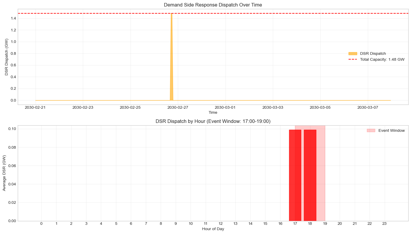
======================================================================
6. DSR Value Analysis#
When does DSR get dispatched? Compare DSR activation with system marginal prices to understand its value.
[7]:
# Compare DSR dispatch with marginal prices
if len(dsr_gens) > 0 and len(n.generators_t.p) > 0 and len(n.buses_t.marginal_price) > 0:
    dsr_cols = [c for c in n.generators_t.p.columns if c in dsr_gens.index]

    if dsr_cols:
        total_dsr = n.generators_t.p[dsr_cols].sum(axis=1) / 1000  # GW

        # Average marginal price across all buses
        avg_price = n.buses_t.marginal_price.mean(axis=1)

        # Create comparison DataFrame
        comparison = pd.DataFrame({
            'dsr_gw': total_dsr,
            'price': avg_price
        })

        # When is DSR active?
        dsr_active = comparison[comparison['dsr_gw'] > 0.001]
        dsr_inactive = comparison[comparison['dsr_gw'] <= 0.001]

        print("DSR VALUE ANALYSIS")
        print("=" * 70)

        if len(dsr_active) > 0:
            print(f"\nPrice Statistics:")
            print(f"  Average price when DSR active: £{dsr_active['price'].mean():.2f}/MWh")
            print(f"  Average price when DSR inactive: £{dsr_inactive['price'].mean():.2f}/MWh")
            print(f"  Price premium captured: £{dsr_active['price'].mean() - dsr_inactive['price'].mean():.2f}/MWh")

            print(f"\nDispatch Triggers:")
            print(f"  Min price during DSR: £{dsr_active['price'].min():.2f}/MWh")
            print(f"  Max price during DSR: £{dsr_active['price'].max():.2f}/MWh")
            print(f"  DSR marginal cost: £{dsr_gens.marginal_cost.iloc[0]:.0f}/MWh")

            # Total value delivered
            total_value = (dsr_active['dsr_gw'] * dsr_active['price']).sum()
            total_cost = (dsr_active['dsr_gw'] * dsr_gens.marginal_cost.iloc[0]).sum()
            print(f"\nEconomic Value:")
            print(f"  Value of DSR (at marginal price): £{total_value:,.0f}")
            print(f"  Cost of DSR (incentive payments): £{total_cost:,.0f}")
            print(f"  Net system benefit: £{total_value - total_cost:,.0f}")

            # Plot price vs DSR
            fig, axes = plt.subplots(2, 1, figsize=(14, 8), sharex=True)

            # Time series overlay
            ax1 = axes[0]
            ax1.fill_between(comparison.index, comparison['dsr_gw'],
                            alpha=0.5, color='orange', label='DSR Dispatch')
            ax1.set_ylabel('DSR Dispatch (GW)', color='orange')
            ax1.tick_params(axis='y', labelcolor='orange')

            ax2 = ax1.twinx()
            ax2.plot(comparison.index, comparison['price'],
                    color='blue', linewidth=1, alpha=0.7, label='Marginal Price')
            ax2.axhline(y=dsr_gens.marginal_cost.iloc[0], color='red',
                       linestyle='--', label=f'DSR Cost: £{dsr_gens.marginal_cost.iloc[0]:.0f}/MWh')
            ax2.set_ylabel('Marginal Price (£/MWh)', color='blue')
            ax2.tick_params(axis='y', labelcolor='blue')
            ax2.legend(loc='upper right')

            ax1.set_title('DSR Dispatch vs System Marginal Price')
            ax1.legend(loc='upper left')

            # Scatter plot: price vs DSR
            axes[1].scatter(dsr_active['price'], dsr_active['dsr_gw'],
                          alpha=0.6, c='orange', s=50, label='DSR Active')
            axes[1].axvline(x=dsr_gens.marginal_cost.iloc[0], color='red',
                          linestyle='--', label=f'DSR Cost: £{dsr_gens.marginal_cost.iloc[0]:.0f}/MWh')
            axes[1].set_xlabel('Marginal Price (£/MWh)')
            axes[1].set_ylabel('DSR Dispatch (GW)')
            axes[1].set_title('DSR Dispatch vs Price (Scatter)')
            axes[1].legend()
            axes[1].grid(True, alpha=0.3)

            plt.tight_layout()
            plt.show()

            print("\n" + "=" * 70)
        else:
            print("No DSR was dispatched during this period")
    else:
        print("No DSR dispatch data")
else:
    print("Marginal price data not available")
DSR VALUE ANALYSIS
======================================================================

Price Statistics:
  Average price when DSR active: £48.36/MWh
  Average price when DSR inactive: £18.78/MWh
  Price premium captured: £29.58/MWh

Dispatch Triggers:
  Min price during DSR: £48.34/MWh
  Max price during DSR: £48.38/MWh
  DSR marginal cost: £40/MWh

Economic Value:
  Value of DSR (at marginal price): £143
  Cost of DSR (incentive payments): £119
  Net system benefit: £25
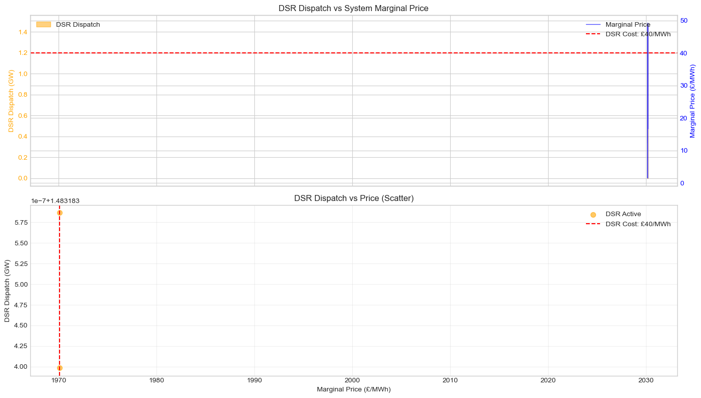
======================================================================
7. Geographic Distribution of DSR#
DSR capacity is distributed across network buses proportionally to peak demand. Let’s visualize this.
[8]:
# Analyze DSR distribution across buses
if len(dsr_gens) > 0:
    # Group by bus
    dsr_by_bus = dsr_gens.groupby('bus')['p_nom'].sum().sort_values(ascending=False)

    print(f"DSR Distribution Across {len(dsr_by_bus)} Buses")
    print(f"  Total capacity: {dsr_by_bus.sum():.1f} MW")
    print(f"  Top 10 buses: {dsr_by_bus.head(10).sum():.1f} MW ({dsr_by_bus.head(10).sum()/dsr_by_bus.sum()*100:.1f}%)")
    print(f"  Min capacity: {dsr_by_bus.min():.2f} MW")
    print(f"  Max capacity: {dsr_by_bus.max():.2f} MW")
    print(f"  Mean capacity: {dsr_by_bus.mean():.2f} MW")
    print(f"  Median capacity: {dsr_by_bus.median():.2f} MW")

    # Plot distribution
    fig, axes = plt.subplots(1, 2, figsize=(14, 5))

    # Top 20 buses
    top20 = dsr_by_bus.head(20)
    axes[0].barh(range(len(top20)), top20.values, color='orange', alpha=0.7)
    axes[0].set_yticks(range(len(top20)))
    axes[0].set_yticklabels(top20.index, fontsize=8)
    axes[0].set_xlabel('DSR Capacity (MW)')
    axes[0].set_title('Top 20 Buses by DSR Capacity')
    axes[0].invert_yaxis()
    axes[0].grid(True, alpha=0.3, axis='x')

    # Histogram of capacity distribution
    axes[1].hist(dsr_by_bus.values, bins=30, color='orange', alpha=0.7, edgecolor='black')
    axes[1].axvline(x=dsr_by_bus.mean(), color='red', linestyle='--',
                   label=f'Mean: {dsr_by_bus.mean():.2f} MW')
    axes[1].axvline(x=dsr_by_bus.median(), color='blue', linestyle='--',
                   label=f'Median: {dsr_by_bus.median():.2f} MW')
    axes[1].set_xlabel('DSR Capacity per Bus (MW)')
    axes[1].set_ylabel('Number of Buses')
    axes[1].set_title('Distribution of DSR Capacity')
    axes[1].legend()
    axes[1].grid(True, alpha=0.3)

    plt.tight_layout()
    plt.show()

    print("\nTop 10 Buses:")
    for i, (bus, capacity) in enumerate(dsr_by_bus.head(10).items(), 1):
        print(f"  {i:2d}. {bus:15s}: {capacity:>8.2f} MW")
else:
    print("No DSR generators found")
DSR Distribution Across 10 Buses
  Total capacity: 1483.2 MW
  Top 10 buses: 1483.2 MW (100.0%)
  Min capacity: 1.83 MW
  Max capacity: 464.72 MW
  Mean capacity: 148.32 MW
  Median capacity: 136.04 MW
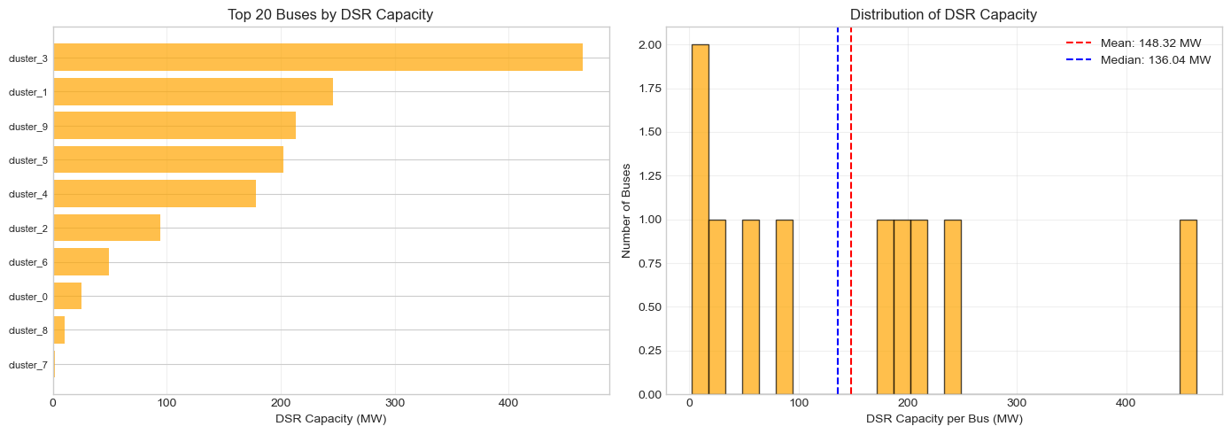
Top 10 Buses:
   1. cluster_3      :   464.72 MW
   2. cluster_1      :   245.88 MW
   3. cluster_9      :   212.92 MW
   4. cluster_5      :   202.15 MW
   5. cluster_4      :   178.11 MW
   6. cluster_2      :    93.98 MW
   7. cluster_6      :    48.91 MW
   8. cluster_0      :    24.77 MW
   9. cluster_8      :     9.93 MW
  10. cluster_7      :     1.83 MW
8. Configuration Reference#
DSR is configured in config/defaults.yaml under demand_flexibility.event_response:
event_response:
  enabled: false                    # Toggle DSR on/off
  mode: "regular"                   # regular, winter, or both
  event_window: ["17:00", "19:00"]  # Peak period (typically 17:00-19:00)
  dsr_capacity_mw: null             # User-defined capacity (MW)
  participation_rate: 0.33          # Fallback: 33% of households participate
  max_reduction_fraction: 0.10      # Fallback: 10% max demand reduction
  winter_months: [10, 11, 12, 1, 2, 3]  # Oct-Mar for winter mode
Key Parameters:#
Parameter |
Description |
Typical Value |
|---|---|---|
|
Turn DSR on/off |
false (opt-in) |
|
Event frequency |
regular, winter, both |
|
Total DSR capacity |
1000-2000 MW |
|
Daily event period |
[“17:00”, “19:00”] |
|
Household participation (fallback) |
0.2-0.4 |
|
Max demand reduction (fallback) |
0.05-0.15 |
|
Winter months for ‘winter’/’both’ modes |
[10,11,12,1,2,3] |
Mode Comparison:#
Mode |
Frequency |
Use Case |
|---|---|---|
regular |
2 events/week year-round |
Baseline flexibility testing |
winter |
5 events/week Oct-Mar |
High winter demand periods |
both |
2/week summer + 5/week winter |
Most realistic scenario |
Capacity Sizing:#
If dsr_capacity_mw is not set, capacity is calculated as:
DSR Capacity = participation_rate × max_reduction_fraction × Peak Demand
For GB with ~40 GW peak demand:
Conservative: 0.25 × 0.08 × 40,000 MW = 800 MW
Moderate: 0.33 × 0.10 × 40,000 MW = 1,320 MW
Ambitious: 0.40 × 0.12 × 40,000 MW = 1,920 MW
The HT35_flex scenario uses 1,500 MW as a realistic mid-point target for 2035.
9. Real-World Context: National Grid ESO Saving Sessions#
PyPSA-GB’s DSR modeling is inspired by real programs like National Grid ESO’s Demand Flexibility Service (“Saving Sessions”):
How Saving Sessions Works:#
Enrollment: Households with smart meters sign up through their energy supplier
Event notification: ESO announces events 24 hours in advance (typically 17:00-19:00)
Baseline establishment: Smart meter calculates typical usage for that period
Demand reduction: Households reduce usage (delay cooking, heating, EV charging)
Reward payment: £3-10 per kWh saved, paid via energy supplier
Winter 2022/23 Results:#
1.6 million households participated
21 events held (Nov 2022 - Mar 2023)
~500 MW average reduction per event
3,300 MWh total energy saved
£50/MWh average cost (vs. £150-300/MWh for backup generation)
2035 Projection (HT35 Scenario):#
5-10 million households with smart meters and flexibility tariffs
1,500 MW achievable reduction (3x current)
50-100 events/year (winter-focused)
Cost-effective alternative to peaker plants and imports
Why DSR is Valuable:#
Avoids generation costs: £50-100/MWh vs. £150-300/MWh for backup
Reduces network stress: Temporal load shifting prevents bottlenecks
Consumer benefits: Households earn rewards for flexibility
Low carbon: Reduces need for fossil fuel peaker plants
Scalable: Can grow with smart meter rollout